I have the following situation. There is a foundation lying on a two layers soil. The Young’s moduli, E_1 and E_2, of the two soil layers are my random variables. The quantity of interest is the maximal settlement U_Y of the foundation under a given load F. Now say that in the deterministic case using mean values of E_1 and E_2 I calculate (with FE software) a settlement of 1 cm. But at the building site I observe a settlement of 1.5 cm. So I perform a bayesian inversion (I first build a PCE on the FE software, very small LOO error) in order to update my probabilistic input. As a result of the bayesian inversion I get the posterior marginals and the correlation matrix. Since the output U_Y is a function of all inputs that feed my FE software/PCE, U_Y \approx f(E_1,E_2), it is logic that my varibles are correlated in order to “match” the observation of 1.5 cm.
Minor remark: I am not sure that one can really rule out thatt the Young’s moduli E_1 and E_2 are correlated for physical reasons: The two soil layers are connected at some interface such that one may have a material exchange between the layers through this interface changing the material properties of the soil near to the interface such that the effective Young’s moduli you seem to use in your computation may become correlated.
I understand and I agree with you, but for your second point only partially. A correlation may exist, but a geotechnical engineer would not assume that there is a correlation between soil parametres of different layers of soil without testing to prove this.
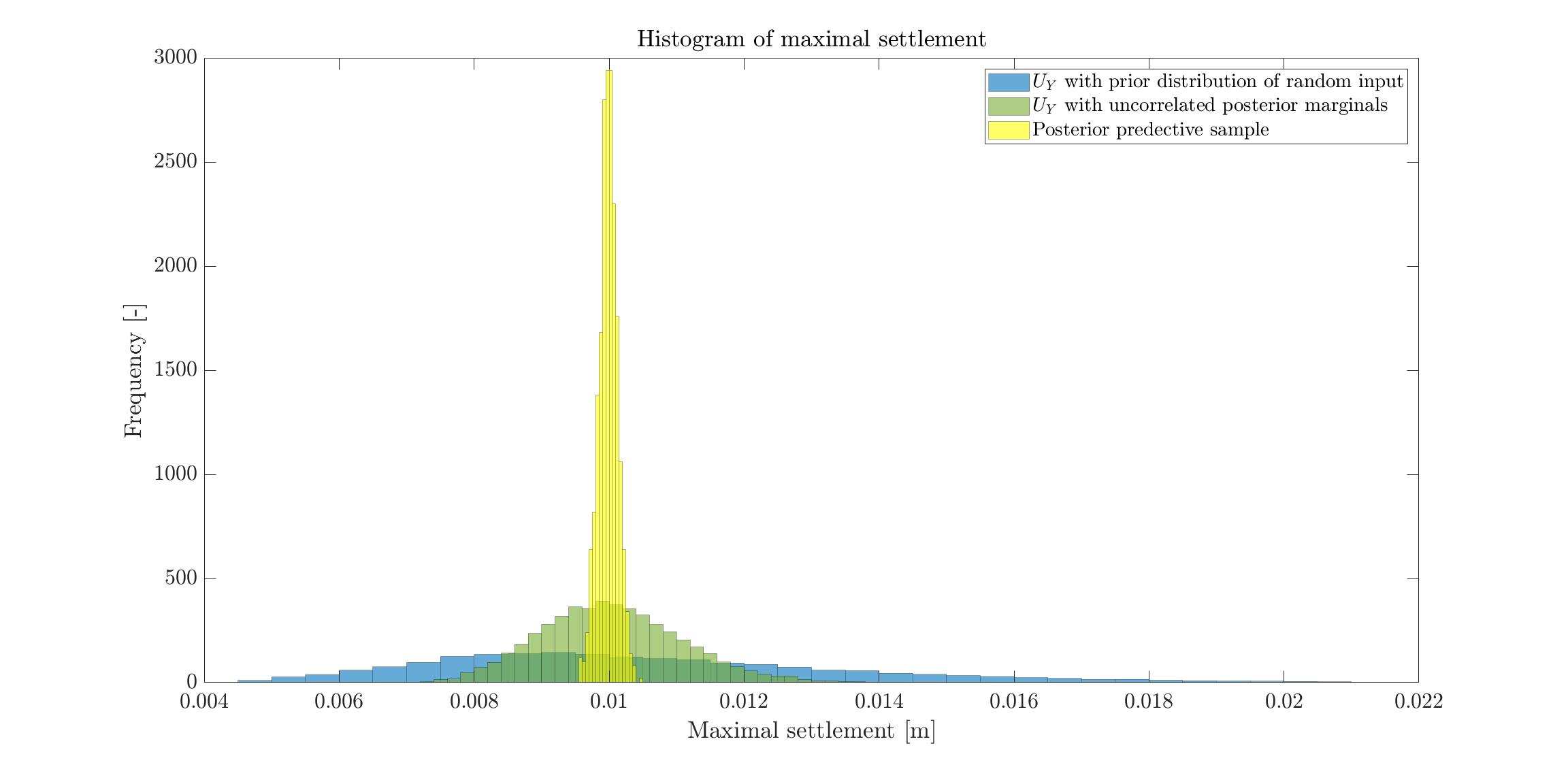
From the client perspective, as shown in the image below, for this specific example using the correlated posterior marginals gives a pdf of U_Y which has less uncertainity with respect to the pdf obtained using the uncorrelated posterior marginals, which means they maybe can optimize the design (and so save money).
Say the threshold of failure is defined as the settlement being bigger than 1.2 cm (NB: the image below shows the foundation example but the observation was 1 cm and in the deterministic case we had about 7 mm), than in the first case the probability of failure is 0%, and the other case about 4%. Assuming a correlation could lead to significantly underestimating the probability of failure, which cannot be accepted.
to avoid that someone gets a wrong impression: It holds in your situation that taking the correlation into account significantly reduces the computed probability for problems, but there are also situations such that ignoring the correlation reduces the computed probability for problems, see e.g. On the importance of accurate models of dependence in UQ: a cautionary tale.
Since your model is (as all models) a simplification of the reality, the computed settlement distribution determined by considering the probability distribution / set of samples with with correlation are only approximations for the values one has to expect in reality, and the same holds for the computed settlement distribution determined by considering the marginal densities. I think that the results determined with correlation should provide the better approximations, but there may be real world situations such that the other results provide better approximations of the reality. Hence, one may consider you considerations as the result of an ensemble computation / ensemble forecast using two sets of random variables as ensemblesand to perform afterwards a worst case analysis of the two results.