Example of Bayesian inference computation creating a model output at the mean of the parameter samples that is outside of the discrete posterior predictive support

Hello,
This is an example for a (incomplete) Bayesian inference computation for a model with vectorial output such that it holds for the model output at the mean of the parameter samples, which is denoted by mean prediction in the plot shown below: It holds for every component that the model output is much larger then the maximum over the values for this component in the samples for the posterior predictive density:

strange_mean_prediction-fig-8 .

I think that this example may be of interest, since in many other example the model output at this mean is contained in the discrete posterior predictive support, such that one expects that this to be a general property, as it is pointed out for example in a contribution in a discussion on UQWorld..

The model output at the mean, denoted by mean prediction in the figure above, is (218.9, 221.239, 224.162, 230.008), For the components of the samples of the posterior predictive the maxima
are (47.9056, 66.6261, 106.543, 171.66).

These numbers and this figure has been generated by the script strange_mean_prediction.m (3.9 KB) that calls the function strange_mean_prediction_func.m (592 Bytes).

To generate this surprising behavior, I used:

1.) A model with a vectorial output and positive model parameters X1 and X2 that is linear with respect to X1 and is in all components a monotone increasing function for X2. This yields that increasing the values for X1 or for X2 increases the values in the components in the corresponding output of the model. It holds for Scr_UQLab_fullsim_ldent_func that the output at (X1,X2)=(X_1,X_2) is equal to

\left (X_1 * (X_2 +0.1),\, X_1 * (X_2 +0.5), \,X_1 * (X_2 +1),\, X_1 * (X_2 +2) \right).

(This model is a surrogate for the model in my real application that also has the discussed properties. Dealing with this model I accidentally created figure in my contributioon to a discusion on UQWorlld .

2.) A data vector that is created from the output of the model for the parameter values
X1 = 5 and X2 = 4 by adding some noise.

3.) For both parameters, a prior is used which is supposed to carry almost no
information and is therefore uniform on [0 200].

4.) After 200 of iterations steps for the MCMC algorithm is holds for the samples
derived after rejecting of the initial 50 percent of the MCMC samples as burnIn values:
On one hand there are still a sufficient number of chains with large values for X1 or for X2, see

strange_mean_prediction-fig-1
strange_mean_prediction-fig-2
but one the other hand the algorithm has already performed a sufficient number of iterations the such the parameters pairs (X1,X2) in the samples create good approximation of the data vector.

5.) The properties of the model now yield that the samples with large values for X1 in general contain a small value for X2 and the samples with large values for X2 in general contain a small value in X1. In the posterior sample scatter plot strange_mean_prediction-fig-7.png one can see
that the sample points for (X1,X,2) are on a line similar to the graph of 1/x on (0,\infty):
strange_mean_prediction-fig-7

6) Now, it holds for the computed arithmetic means from the samples and the data pair that was used to created the to be approximated that the mean of 5.8 for X1 is slightly larger then the value of 5 used for the data creation and that the mean of 37 for X2 is much larger then the value of 4 used for the data creation. Considering the marks in the scatter plot above indicating the position of these means, one observes that both mean are larger then position of the the maximum of the corresponding discrete sample density:

Since the model output is linear in X1 and almost linear in X2, we see that this yield that the components of the model output for this mean value pair, i.e. the mean prediction in the first plot, are therefore much larger then the components of the model output at (5,4). Since the considered data vector is a noisy version of this model output and is approximated by the samples of the posterior predictive distribution, we get maximal values for the components that are smaller then the components
of the model output at the mean.

Remark: If one is replacing the mean by the maxima of the a posteriori density (MAP), being
equal to (5.6, 3.4) in considered situation, one can mark it in the scatter plot by the red cross in the (X1,X2) plot:
strange_mean_prediction-fig-4

Marking in the it in the posterior density plots the model output at the MAP value by map prediction,
the result is is less surprising then the plot above:
strange_mean_prediction-fig-5

2 Likes

Hi Olaf

Thanks for this great example of when not to rely on the posterior mean! Because of the product interaction of X_1 and X_2 and the overlapping prior distributions, the forward model can return identical predictions for arbitrary parameter combinations as long as

X_2 = \frac{c}{X_1}, \quad c\in\mathbb{R}.

This is an example of an extremely ill-posed inverse problem! This hyperbolic relation can be seen in the bivariate posterior marginal of X_1 and X_2. The center of the posterior marginal’s probability mass then naturally lies outside its support.

Such problems can be difficult for many MCMC samplers (not AIES) because their acceptance ratio becomes extremely small once the chains get stuck in the hyperbolic trench. It is therefore often easier to reparametrize the problem using:

\xi_1 = X_1\\ \xi_2 = X_1\cdot X_2

to obtain

\{\xi_2+0.1\xi_1; \xi_2+0.5\xi_1;\xi_2+\xi_1;\xi_2+2\xi_1\}

\xi_2 does not follow the same probability distribution as X_2, but the transformed model no longer exhibits a hyperbolic relation between its two parameters as shown in the inverse analysis I did with this transformed model:

PosteriorDistTransformed

The highlighted point is the posterior mean that clearly lies well inside the posterior support.

2 Likes

Dear Paul,

thanks for your answer with this elaborated discussion and your suggestion to reparametrize the problem. I will apply this to my real world application.
I view of your remark that the AIES MSMC samplers has less problems with the hyperbolic trench as other MCMC smaplers I would like to point out some observation that surprised me somehow:

Since I believed that the model output at the mean of the parameter samples would be in the discrete posterior predictive support if the numbers of steps became sufficiently large, I increased the value of Solver.MCMC.Steps up to 25,000, but could not observe this behavior. This behavior was still not observed after I increased Solver.MCMC.Steps even further to 250,000. After more the 72 hours of computing time got I the following plots for the MCMC samples with a strange observation in the second plot, i.e. the one for X2:

strange_mean_prediction_more_steps-fig-1

strange_mean_prediction_more_steps-fig-2

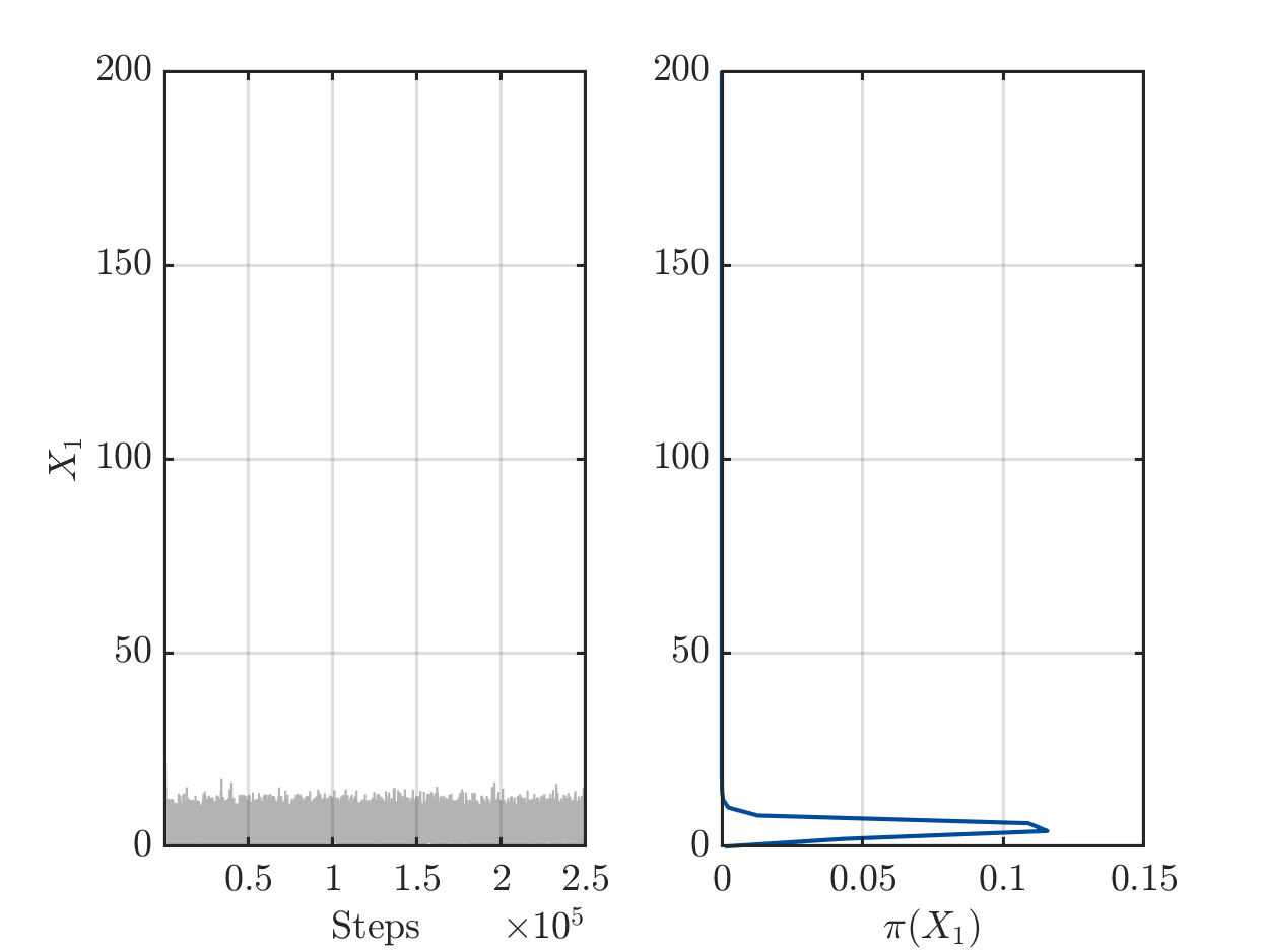
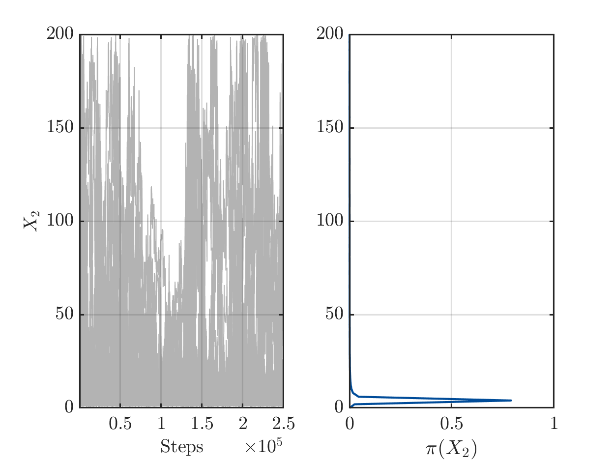
I try to figure out if this change of behavior for the samples for X2 at around step 110,000 can be a real result of the algorithm or if it may be an indication that there may be some well hidden error somewhere?
What do you think?

Many thanks again

Greetings
Olaf

Hi Olaf

Are you referring to the fact that some MCMC chains of X_2 are moving towards the upper support limit (200) after initially moving towards the lower support limit (0)?

I think this is perfectly normal and can in fact be expected. The MCMC algorithm in the uniform prior case is exploring the domain solely based on the likelihood function. Considering the hyperbolic relation I mentioned in my previous post, there are points all along this trench (also with small X_1 and quite large X_2) for which the likelihood returns the same value. The AIES algorithm finds those points reliably while I am not sure the Metropolis-Hastings algorithm would have an equally easy time doing so.

Dear Paul,

yes, I as referring to the fact that up to step 110,000 there seemed to be a tendency for the X_2 values in the MCMC chains to move the the lower support limit but that after step 130,000 there were again chains with large values for X_2.

I agree that the model returns quite similar predictions on the trench of X_2 = c/ X_1, but they are not completely identically since the model perdition on this trench would be

\left ( c+ 0.1 * X_1 , c + 0.5 X_1 ,c + X_1 , c+ 2X_1 \right).

I believed that this would some create a drift on the trench such that X_1 and therefore also X_2 would converge at the end, but it seems that I was to optimistic.

To ensure that the above observation this is really a result of my ill posed formulation of problem and not of some hidden bug, I have considered my problem with your suggest transformation of variables and started a UQLab run with Solver.MCMC.Steps being 250.000 as run over the weekend. I stopped after 56 hours of computing time with AIES announcing that 87 % of the computing in complete. The resulting plots for the MCMC sample do not show any strange blow until step 210,000, i.e. they confirm that the above observation results from my problem formulation:

no_strange_mean_predictio-more-stepsn-fig-1 no_strange_mean_predictio-more-stepsn-fig-2

Greetings
Olaf

1 Like