Dear UQLab community,
I have recently done a Bayesian inversion with UQLab, in the following context :
-
Model : ZSoil (finite element software, surrogated by an accurate PCK)
-
Two inputs : a construction parameter \lambda (which depends on how quick is made the construction) and a soil parameter E (Young’s modulus).
-
Output : the settlement of the ground, computed by ZSoil
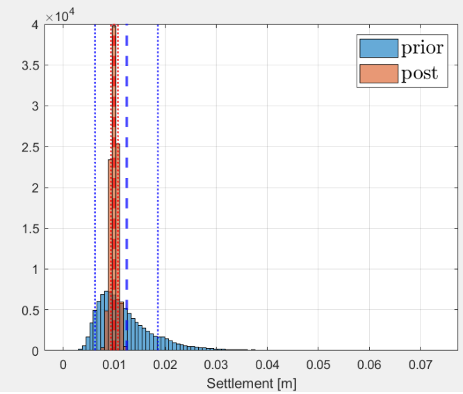
As the discrepancy is small, I reckoned the standard deviation of the posterior predictive would be quite small (with an accurate measurement, not very probable, I think the uncertainty tends to decrease).
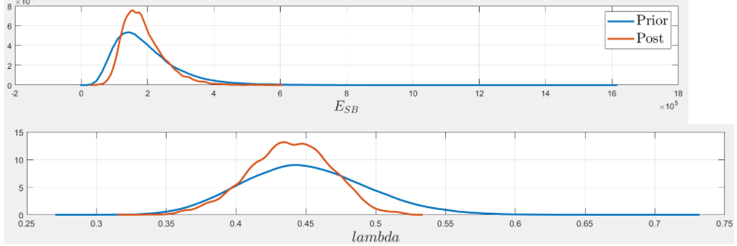
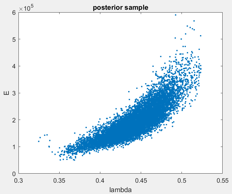
Actually, the standard deviation of the posterior predictive is quite small, but the inputs are almost as much uncertain as before. I mean there is not much reduction in the uncertainty of \lambda and E. I think the inference has created a correlation between my inputs, which prevents from extreme outputs. That is to say the coefficient of variation of the output has been reduced much more than the CoV of the inputs.
Here is the posterior predictive :
The thing is, there should not have a correlation between E and \lambda, because it does not have a physical meaning.
Thus my question is : is there a way to prevent the posterior inputs to become correlated ? To put it another way, is it possible to restrain the MCMC to uncorrelated values ?
Thanks a lot,
Marc
Dear Marc,
My short answer: I think that you can not restrain the MCMC to uncorrelated values since the results of the Bayesian Inversion will be correlated since they are all model inputs leading to model outputs being approximation of the observations.
More details: .
I assume that you also had some value for the settlement S_{observ} that is considered as observation in the formulation of the Bayesian inverse problem. And it holds somehow (simplified) that the sample pairs for (\lambda_i,E_i) created by MCMC- computations satisfy that the corresponding output of the model, i.e. the settlement for all these data pairs are good approximations of the “observed” settlement. (If you have several observed settlements, you have (less) goood approximations for all of of them).
Moreover, I assume that you are in the situation that increasing \lambda and keeping E fixed will either increase or decrease the model output while increasing E and keeping \lambda fixed will change the model output in the opposite way. I suggest that you to check this.
Now it follows if you have two input pairs (\lambda_1,E_1) and (\lambda_2,E_2) generating model outputs both being good approximations for S_{observ} it yields that the model outputs for both data pairs will be almost the same. Hence, it follows that the difference in the model output consierding the data pairs (\lambda_1,E_1) and (\lambda_1,E_2) has to be partially compensated by the difference between the data pairs (\lambda_1,E_2) and (\lambda_2,E_2), e.g. if first difference is positive the second difference will by typically negative. And since I assume that you have opposites monotonically behavior of the model output with respect to \lambda and E this yields that you will have typically that E_2 -E_1 and \lambda_2 - \lambda_1 have the same sign, generating/explaining the observed correlation.
I am not sure but it seems to me that you assume in your Bayesian inversion problem that the discrepancy in the problem is already known. It this is correct, I suggest to consider the situation wherin is discrepancy is also an unknown quantity. I think that this will change the posterior uncertainty in E and \lambda also.$.
Greetings
Olaf
Dear Olaf,
Thanks for your reply. I didn’t want to post an incomplete answer, so I’ve thought a lot about this.
You perfectly understood my Bayesian inversion, and the compensation between E and \lambda. Thus I reproduced an analytical fictitious example on the model f(x,y) = x-y. An observation f_i leads here to a huge correlation between X and Y.
That being said, our main problem is the posterior correlation, between a priori independant inputs. In our former example, the correlation between E and \lambda should not exist a priori, because it has not a physical meaning. It can seem strange that because of an observation, a correlation appears.
I think there is a kind of confusion here, because after the observation, we focus on the distribution given the observation, which is a different couple of variables than the prior one. I mean we don’t focus on (E,\lambda) anymore, but on (E,\lambda \vert S_{observation}) which has different properties.
To conclude, I think the correlation between the posterior inputs is relevant, even if the assumption of independent prior inputs is made.
Finally, we do not use unknown discrepancy for now. I assume it does not help understanding the inversion, and can sometime hide some issues. Do you recommend the use of unknown discrepancy, especially when you can’t put numbers on its value (see my former post Bayesian inversion : discrepancy) ?
Thanks again,
Marc
Dear Marc,
to maybe reduce your confusion I would like to present my private interpretation of the results of Bayesian inversion, following with modifications
J. Kaiiop, E. Somersalo, “Satistical and computational inverse Problems”, 2004, Sec 3.1:
- Ignoring that your model (as all models) is not a perfect representation of the reality, I assume that there is an fixed, but unknown true parameter pair (E_{true},\lambda_{true}) such that the real world measurements (=observations) are equal to this model output with some added noise (i.e. model bias is ignored here!).
- Before one deals with the observations, one had derived a continuous random variable (E_{priori},\lambda_{prior}) representing all information/guesses/beliefs/expert opinions that one had on the pair (E_{true},\lambda_{true}) before the observation S_{observation} had been made/had been evaluated.
The density of (E_{priori},\lambda_{prior}) is the prior density. In your considerations, the components of (E_{priori},\lambda_{prior}) are independent, such that the prior density is the product of the prior densities for E and \lambda.
- Now, one is considering S_{observation} as an output of the model (with added noise) for a sample for (E_{priori},\lambda_{prior}). By following Bayes’s theorem one gets a formulae for the conditional probability distribution (E_{prior},\lambda_{prior} | S_{observation}) and by using UQLab, one gets a set of samples for this distribution, as shown in your first post.
- This conditional probability distribution (= posterior distribution) expresses what one can deduce about (E_{true},\lambda_{true}) by combining the information encoded in the prior densities and the observation S_{observation} of the model output with noise (i.e. discrepancy) . Hence, one should use this conditional probability distribution for the computation in the following, i.e. one should focus on (E_{prior},\lambda_{prior} | S_{observation}) with its “different properties” as the prior distribution.
Concerning using an unknown discrepancy: Especially if you do not know the value for the discrepancy I would suggest to use an unknown discrepancy, even if the formulation of the Bayesian inverse problem get more complicated. If you work with a know discrepancy you have to provide the value. If this value is too large, the likelihood function may become to flat such that the MCMC algorithm may produce samples set with an uncertainty that may be too large. Hence, one may have to play around with the provided value for the discrepancy and have to check if this inflects the uncertainties in E and \lambda, and may have to try to find an optimal value for the discrepancy.
By using an unknown discrepancy, one expects (or al least hopes) that in the resulting sets of samples the value discrepancy is automatically chosen as an approximation of the optimal value and that the uncertainty in E and \lambda may be optimized.
Greetings
Olaf
,
Dear Olaf,
Thanks for your summary of the Bayesian procedure. It clearly puts into words the inversion steps.
I think I understand your stance on the unknown discrepancy. Don’t you think it can lead to the update we’d like to have, rather than the real one ? I mean I wonder if the unknown discrepancy does not overestimate the information contained in the observation. Maybe a huge but known discrepancy will give more conservative posteriors ?
Thanks for your answers, it helps a lot,
Marc
Dear Marc,
Just a remark: Be aware that the point of view in step 1,2 and 4 of my interpretation will not be approved by all UQ-experts, I already had some discussions about this.
The question is somehow what is the real update? Using a huge but know discrepancy yields that during the computation of the likelihood the error, i.e. the difference between model output and observation is divided by a large number such that the sum in the exponent of the becomes small, such that at the end the likelihood gets small variations… and at the end the update may be to small / to conservative.
I would suggest to use an unknown distribution, such that the largest possible value for he distribution if sufficiently large. I think that the default reaction of UQ-Lab (see Sec 2.2.6 of the manual) could be a start , i.e. the discrepancy is an additive Gaussian discrepancy term (with mean 0) and variance \sigma^2 and the prior distribution for \sigma^2 is the uniform distribution \mathcal U(0,\mu^2) with \mu being the empirical mean of the observed values (okay this maximal value is very large.)
It is my opinion that one can trust the result of computation with an unknown discrepancy if the omputed values for the discrepancy do not accumulate near to the maximal possible value. If they accumulate in this way, I would suggest to increase the maximal possible value and the re-perform the MCMC computations, even if this violates the rule that the prior should fixed before the measurement is done/ the measured value is used for further investigations.
Greetings
Olaf
Dear Olaf,
It is really interesting. I’ll do some research and try some tests in this direction.
Thanks,
Marc