Thank you for developing such an amazing software for us to use.
I want to use the PCE module to get a surrogate where the experimental design is specified manually (as in the attached files, with three inputs and on output; train_data for training, test_data for validation; train_data(:,1:3) the inputs and train_data(:,4) the output, same goes for test_data). Since the distributions of the input random variables are unknown, and the use of PCE requires the information of distributions. So the statistical inference module available in UQlab is used to get the distribution info from the data set, the result is: input 1~uniform (0.1 2), input 2~Beta (0.6983 1.951 0 1), input 3~Gamma (0.3048 666.879).
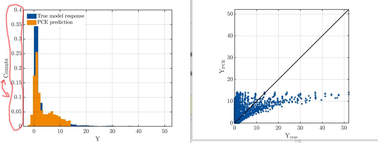
To this end, I can use the PCE to construct the surrogate model. And based on my own experience, the PCE can generally yield a good approximation to the original model. But I don’t know why it doesn’t work in this way for this example, i.e. the PCE is poorly behaved with quite high LOO error and validation error, and can hardly get a good prediction of the new samples in the domain, even with high polynomial degree. And the histogram plot does not seem to be correct since the value in vertical is decimal, which should be an integer (as shown in fig). I wonder if anyone can help me check with that and find the reason why the PCE doesn’t work for my case. Really appreciate your kind help.
BTW, after get the PCE using UQlab, how can I get an explicit expression of the PCE surrogate (the relation between the coefficients and the multivariate orthonormal polynomials)? how to interpret the myPCE.PCE.Basis.Indices sparse array in the result?
Attached is the data set (training and testing), and the code I used.
I’m a new user and cannot upload attachments, could you please give me access to do that? Many thanks!
The uq_histogram displays normalized values by default (see UQLib user manual, page 77). This way, you can plot several histograms with different numbers of points into the same figure. To get the raw counts, use the additional argument 'Normalized', false.
The method you describe to get the distributions of your input random variables sounds correct. How good is the fit of the fitted distributions? To make sure the fit is reasonable, you could plot the histograms of the input data together with the fitted distributions. If you have any additional information on the input distributions (bounds, mean, etc), you can help the inference module by specifying them (see Inference manual, section 2.1.2).
Now, assuming that the input distributions are appropriate, it does not follow immediately that the PCE approximation is good. PCE works well if your model is smooth, but if it is discontinuous or has kinks, it won’t provide a good approximation. Also, if your model is very complex, it might be that many PCE terms are needed to get an accurate approximation, which in turn requires a lot of experimental design points. Are you using sparse regression (LARS)? Can you afford to use more points for training? Try to use a higher degree, possibly restricting the interaction order to 2.
For the explicit expression of the PCE surrogate: myPCE.PCE.Basis.Indices is a sparse matrix. To see the matrix in the usual full form, use A = full(myPCE.PCE.Basis.Indices).
Every row contains one multi-index, each characterizing a basis function. myPCE.PCE.Coefficients is the corresponding vector of coefficients. Its i-th entry is the coefficient belonging to the basis function/multi-index in the i-th row of A.
Note that UQLab automatically transforms the input distributions into standard distributions, as described in another post.
In my case, I have more than 6000 samples with only three input random variables, so I can afford using full PCE with a high degree instead of the sparse one. I think I’ve found the reason now. Using UQlab statistical reference, the distribution type of input three is Gamma ~[3.048e-01(a), 6.669e+02(b)], the corresponding first two moments are 2188 (b/a)and 84.73(sqrt(b)/a), respectively. However, the moments of the sample is actually 203.26 (a*b) and 368.18 (sqrt(a)*b), and this is consistent with the equation found in Wikipedia. So, I think the moment calculation equation in UQlab statistical reference for Gamma distribution may need to be modified to get the correct one (forgive me if I was wrong ). After I modified my InputOpts using the correct moments (203.26 and 368.18), the fitting result is much better. But still, the PCE may not very suitable for my case (the RMSE is large), since the distribution information needs to be inferred from the data.
Anyway,your reply is really helpful, and I think I can get the explicit formula of PCE now according to your information, thanks and best regards.
You are pretty close to be able to upload files! You just need to browse around UQWorld a bit more and read a few more posts . You’ve read 14 posts so far; you need to read 30[1].
Once you do that, you’ll be notified that you’re granted Basic User and be granted an access to upload attachments (\leq 4MB).
If you’re curious about how UQWorld trust level works: you additionally need to have visited 5 topics and spend a total of 10 minutes reading something here before you can start uploading files. But you’ve done these other two already! ↩︎
The Gamma distribution in UQLab is parametrized by shape parameter k and scale parameter lambda (see uq_gamma_pdf.m), so with the corresponding formulas, you should obtain the correct moments – you can e.g. use UQLab’s function uq_gamma_PtoM to compute the moments of your Gamma distribution from given parameters. If that doesn’t give the right moments, could you upload your data set so that we can have a look whether there is indeed a bug?
Regarding full vs sparse PCE – normally it does not make sense to use OLS instead of sparse solvers like LARS. But indeed, if you have more than 6000 points in only three dimensions, this is more than enough to do OLS even with degree 20 or more.
Have you tried to check how well your fitted distributions describe your data? Other than that, reasons for the poor fit could be:
the model is not smooth at all
there is an additional source of randomness (noise), i.e., your model might return different values even when run twice with the same input parameters (see Xujia’s post on stochastic simulators)
Good luck with your research, let us know when (and how) you found a way to surrogate your model!
Thanks for the post. The parameterization of a Gamma distribution in UQLab is different from that in Matlab, as you can find two possible parameterizations on Wikipedia. Such a difference is explained in some functions, e.g. uq_gamma_pdf (you can read it by typing help uq_gamma_pdf after activating uqlab). The inference module uses the built-in Matlab function fitdist, which results in the parameters of Gamma distributions defined in Matlab. However, the conversion to the UQLab setting is not performed automatically, which leads to an inconsistent problem. We recently found this problem, and it will be fixed in the next release.
What you have done (using the sample moments in your input option) is to use the method of moments to infer the parameters for Gamma distributions, which is one way to solve the problem. Alternatively, you can also use the inference module and then manually transform the inferred parameters to the UQLab setting. Consider an input object myInput created by the inference module. A new (correct) input object can be created by
clear InputOpts
for i=1:length(myInput.Marginals)
   InputOpts.Marginals(i).Type = myInput.Marginals(i).Type;
   p = myInput.Marginals(i).Parameters;
   if strcmp(myInput.Marginals(i).Type,'Gamma')
       %this step changes the parameters
       InputOpts.Marginals(i).Parameters = [1/p(2),p(1)];
   else
       InputOpts.Marginals(i).Parameters = p;
   end
end
NewInput = uq_createInput(InputOpts);
Note that if you want to use copulas, you should either set it up for the new input object or infer it again from data by specifying the marginal distributions (please see the inference manual for details).
Could you please try this method and see if you get a better fit? Indeed, your current setting should also circumvent the problem of inconsistency, and you reported that the results are not so convincing. I think what @nluethen suggested in her last answer is very helpful.
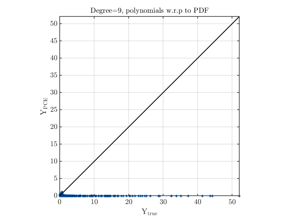
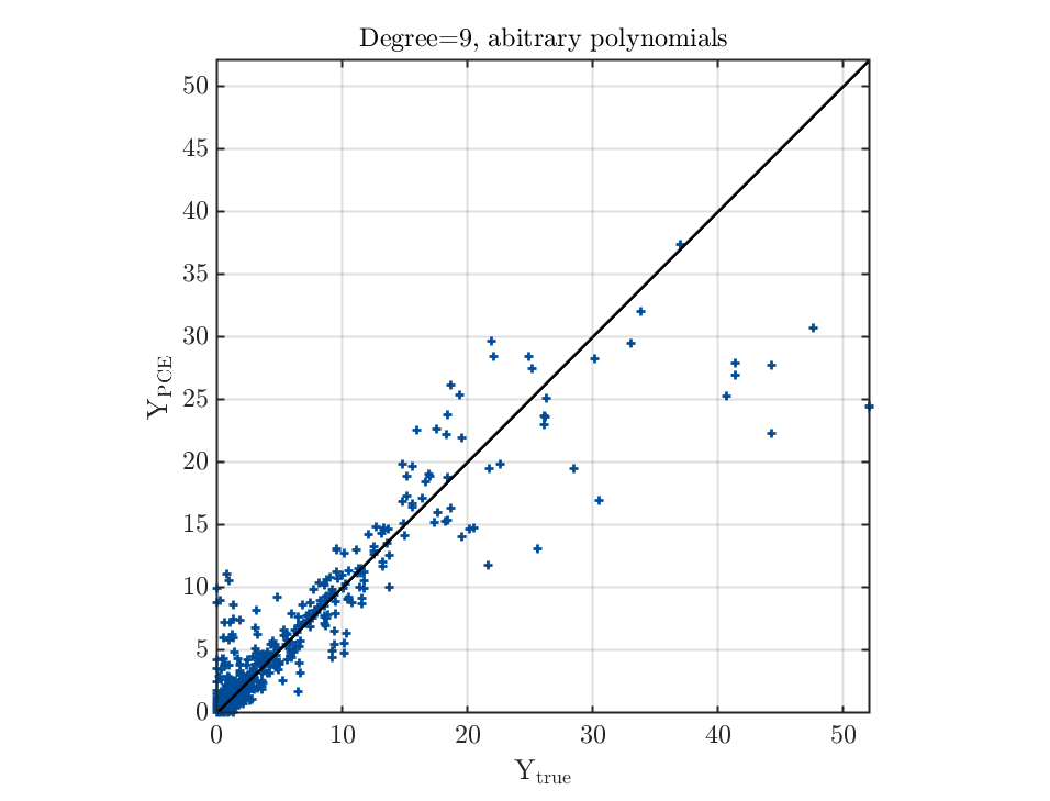
Thank you for helping me solve the problems when using UQLab. But I still cannot fully follow your suggestions to get a satisfactory result, e.g. how to check the smoothness given a set of points? And I found that using the orthonormal polynomials corresponding to the input distributions yields poor performance of PCE, whereas using the arbitrary ones can get better results.
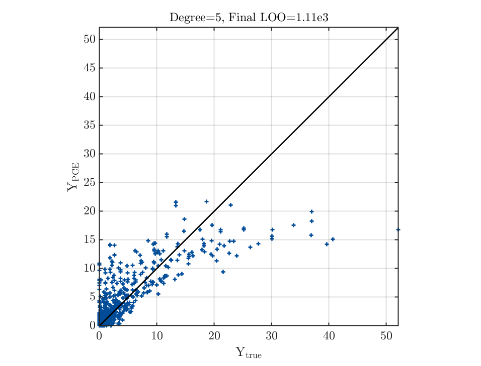
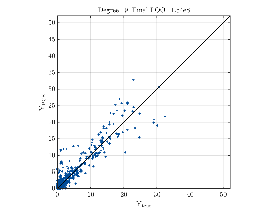
Also, it looks like the corrected LOO error (Final LOO error estimate) increases with the maximum polynomial degree for the same problem, even I have enough data, but the fitting does not necessarily get worse for a large degree (most of the time better result can be obtained with a larger degree, although the accuracy is still poor). Is there any reason behind this?
It is hard to describe my problem clearly, so I will just attach my data (the first three columns are the inputs,fourth is the output) along with the source code, hope you can help me check with that, really appreciate it.
First of all, with the help of your feedback, we figured out another problem in the code related to the setup of PCE for Gamma distributions. This explains why in your case arbitrary PCEs work but analytical orthogonal polynomials (more precisely Laguerre polynomials) with respect to the input distributions do not. This problem will be fixed in the next release. By the way, arbitrary PCEs and analytical orthogonal polynomials for common parametric distributions (e.g. normal, uniform) are equivalent.
For analyzing the data, I would like to share some ideas:
The input values (at least the first two variables) are generated from grids rather than random sampling. This can cause some potential problems because the statistical inference usually assumes that samples are independent realizations of a probability distribution. As deterministic designs (except quasi-random samples) are not representative of the underlying distribution, I would recommend you to specify the distribution (according to the physics or expert knowledge) instead of using the inference to calibrate the distributions. I would like to also remark that your input variables are not independent.
Because the input values do not come from the inferred distributions, the matrix \Psi^T\Psi can be ill-conditioned. Recall that the OLS solution
\hat{\boldsymbol{\beta}} = (\Psi^T\Psi)^{-1}\Psi^T\boldsymbol{y}
, and thus a singular \Psi^T\Psi can lead to severe numerical problems. With the provided data, I tried to manually invert the matrix \Psi^T\Psi and Matlab raised a warning
Warning: Matrix is close to singular or badly scaled. Results may be
inaccurate. RCOND = 9.184018e-17.
When checking the leave-one-out error, especially when \Psi^T\Psi is close to singular, please use the standard leave-one-out error (so not the modified one). You can, of course, enable the option ModifiedLoo = 1 to perform model selections. However, the unmodified leave-one-out error gives you the correct cross-validation error (this quantity is stored in myPCE.Error.LOO). Then, you can see that It gives a much reasonable estimate of the error.
I did some preliminary analysis of your data and it seems to me that the data are smooth but have a strong local behavior: for most of the input parameters, the output has small values, whereas large output values are localized on the boundary X_1 \in [0.5,1.5]X_2, X_3=0. This local and boundary behavior might be difficult to be captured by a global approach, such as PCE (more advanced techniques may be more appropriate). Anyway, I manage to have an average R^2 (defined in your code) over 0.92 by using high degree polynomials:
Because the matrix \Psi is not “well-conditioned”, LARS is only able to slightly improve the results.
In a nutshell, from a pure data analysis perspective, I think the experimental design is not very suitable. If you can re-run simulations, I suggest paying more attention to the experimental design (if there is a physical justification for the current data, it is fine).

 ). After I modified my InputOpts using the correct moments (203.26 and 368.18), the fitting result is much better. But still, the PCE may not very suitable for my case (the RMSE is large), since the distribution information needs to be inferred from the data.
 . You’ve read 14 posts so far; you need to read 30