In this post, we are going to discuss stochastic simulators, a relatively new concept arising in engineering. In fact, such simulators have been widely applied in many other fields for decades, such as economics, finance, and epidemics. The aim of this discussion is to give a clear overview of the concept of stochastic simulators with a focus on various applications. Furthermore, the necessity of developing surrogate models for such simulators will be briefly introduced.
What is a stochastic simulator ?
Simulators are computational codes that are developed to mimic the behaviour of complex systems or model real-life situations. With the increasing computational power, simulators are nowadays used in virtually all fields of applied science and engineering to study the modelled scenario and make predictions about the system performance. For example, if we want to understand the mechanical behaviour of an aircraft under some extreme climate condition, a finite element model can be created to analyse its resistance to environmental loads, instead of resorting to expensive experiments.
More precisely, a simulator can be considered as a function which maps a set of input parameters to the output quantity of interest. For instance, a finite element model for structural analysis takes the loads and material properties as input and produces the displacement-, strain and stress fields as output QoI. Depending on the nature of the QoI, two classes of simulators are usually observed in practice. The first one is the so-called deterministic simulator: deterministic in the sense that repeated runs of the simulator with the same input parameters provide exactly the same value of the output QoI. In contrast, stochastic simulators return different results when run twice with the same input parameters. In other words, the QoI of a stochastic simulator is a random variable.
The random nature sounds a bit weird. Where does the randomness come from? To figure it out, the modelled process is worth a detailed analysis. In fact, a stochastic simulator is based on a deterministic one, since computers (so far…) are deterministic machines. However, the input variables that uniquely determine the QoI are either not fully accessible or have too high a dimension to work with. In the former case, the modelled scenario itself is stochastic due to lack of knowledge (we cannot specify all the relevant input variables), so random seeds are introduced inside the simulator on top of the input parameters to reproduce the randomness within a deterministic framework. In the case of high dimensional input, the problem is usually intractable, so only a few “important” parameters are kept in the study by letting the others as “noisy” variables. Consequently, when we only control a part of the input parameters and let the others vary in their range of definition, the output becomes random.
Examples
Despite its weird behaviour, stochastic simulators are widely used in many fields. Let’s look at some typical examples.
Wind turbine design
In the wind turbine design process, the structural components need to be analyzed under different combinations of environmental loads to access its performance and reliability. Therefore, the simulation consists of two parts: generation of the external excitation (wind inflow) and the aero-servo-elastic simulation referring to the complex multi-physics scenario including mutual interactions of wind inflow (and possibly waves, in case of offshore structures), aerodynamics, hydrodynamics, structural dynamics (elastic deflections) and control systems.
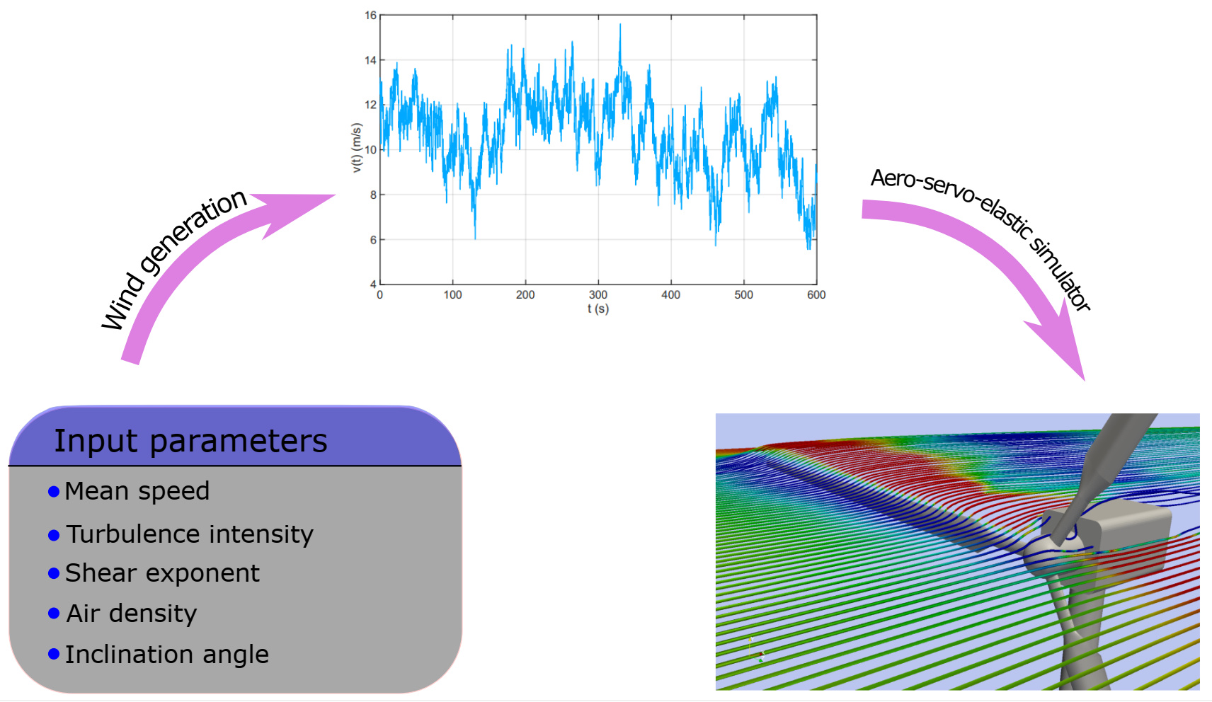
Figure 1: General scheme for wind turbine simulations
In the generation phase, the simulator takes some macroscopic values as input such as the mean speed of wind, turbulence intensity, profile with height, etc. However, these synthetic values cannot uniquely determine a wind field. Therefore, the generator uses random seeds on top of the well-defined characteristic variables to have a coherent inflow, which is usually based on the power spectrum density.[1] Although the aero-servo-elastic simulation is deterministic with respect to the generated inflow, considering both simulations with the macroscopic descriptors as input parameters, the wind turbine simulator is stochastic: a single realization of the three parameters listed above leads to different realizations of the wind field, and thus to different structural performance.
Stock pricing model in Finance
In finance, a stock represents a share in the ownership of an incorporated company. Stocks are issued by a corporation in the market, and investors buy stocks anticipating that it will yield income from dividends and appreciate, or grow, in value. In financial markets, the dynamics of stock prices are reflected by fluctuations of their price (or value) over time, denoted by S_t (referring to the value at time t). The stock price is affected not only by complex interactions inside the market but also by politics and external hazards, and thus it is almost impossible to propose a deterministic model regrouping all the relevant factors together, which gives precise insights of the evolution of stock price. Therefore, S_t is modeled as a stochastic process to represent its random nature.

Figure 2: Evolution of the price of Alphabet (Google) stocks
The mathematical equation that is broadly used to simulate the evolution of stock price is the geometric Brownian motion, expressed by the stochastic differential equation
where \mu is called drift, which denotes the expected return per unit stock per unit time, \sigma is called volatility, which measures the stability of stock price, and W_t is a Wiener process (a.k.a. Brownian motion), which represents unexpected hazards perturbing the price.[2]
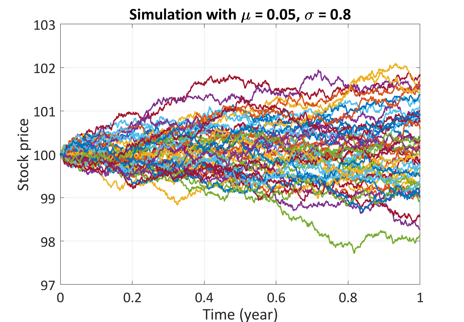
Figure 3: Trajectories of a geometric Brownian motion
The equation implies that with a fixed drift and volatility, S_t can have different profile due to different realizations of W_t, and thus the return for a certain time period is a random variable. Thanks to the simplicity of the equation, the analytical solution can be derived with the help of Itô’s calculus. Nevertheless, more complex pricing models are used in practice (e.g. the Heston model), where closed-form analytical solutions are generally not available, and the associated stochastic differential equation can only be solved numerically.
Epidemics
One of the key topics in epidemics is to study the spread of infectious diseases, which helps carry out necessary operations to minimize the social and ethical impacts during the outbreak. Similar to the previous example about the stock price, the process is rather complex: it depends highly on the interactions among individuals after the outbreak and the recovery ability of each infected individual.
Deterministic simulators have been proposed to represent the spread scenario, especially the susceptible-infected-recovered (SIR) model. Despite the well-established deterministic models, stochastic epidemic models have shown diverse advantages.[3] The standard stochastic SIR epidemic model is a simple extension to the deterministic model: the contacts among individuals are random in time, and the recovery time of each infected individual is also random.
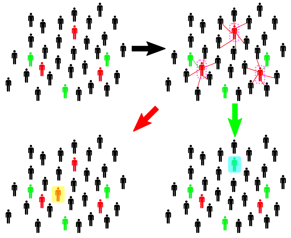
Figure 4: Sketch of the SIR model
The procedure is illustrated in Figure 4 above: susceptible individuals are marked as black, while infected and recovered individuals are red and green, respectively. We will summarize some important aspects without going into the details. For a given configuration of individuals, the next configuration has two possibilities: either one susceptible individual gets infected (highlighted in yellow) or one infected individual is recovered (highlighted in cyan). The evolution depends on which state comes first in time, where both occurring times are described as random variables. As a result, for a given initial configuration, the dynamics are stochastic.
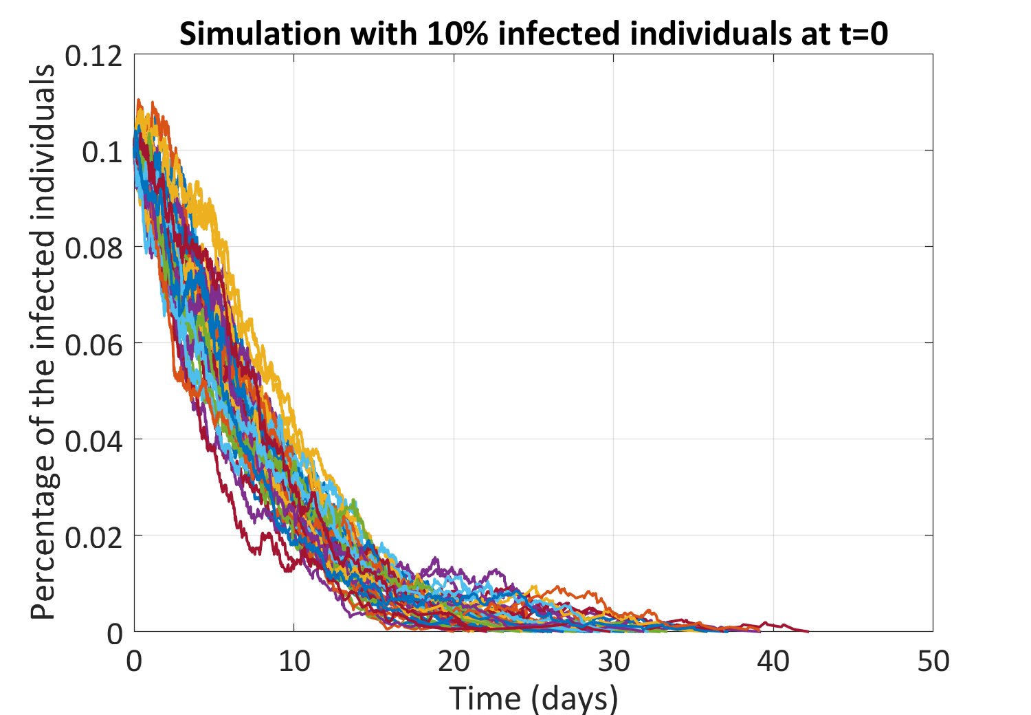
Figure 5: Sample trajectories of the fraction of infected individuals
Why surrogate models of stochastic simulators?
As it is well known, high-fidelity simulators can be very costly to run. Due to their random nature, stochastic simulators should be repeatedly run many times with the same input parameters to fully characterize the output QoI, which is a probability distribution. Moreover, in the context of robust design, we may want to find the best design parameters to optimize certain functions, such as the expectation of the output QoI.
An appropriate way to alleviate the burden is to build a surrogate model (a.k.a. emulator), which mimics the original computational model but requires much fewer computation resources. Conventional surrogate modelling methods such as Gaussian processes[4] and polynomial chaos expansions[5], which have been successfully developed for deterministic simulators, cannot be directly applied to stochastic codes due to the random nature of the latter.
Summary
Stochastic simulators are computational models that have intrinsic randomness and are used to model complex stochastic scenarios. As a result, each model evaluation for given input parameters produces a realization of a random variable. Despite the arbitrary definition, stochastic simulators are ubiquitous: whenever all the relevant input parameters that uniquely determine the output cannot be fully specified, the output of the model will be uncertain. They are present in various fields, among others, engineering, finance, and epidemics.
Unlike deterministic simulators, surrogate modelling for stochastic simulators is still in its infancy. The development of appropriate stochastic emulators will provide a more efficient way to quantify uncertainty within complex systems: the low-cost surrogate models can be run as many times as desired with reasonable computational resources. Therefore, it will allow engineers to optimize the behavior of structures and help assess potential risks for decision making.
Back to the Chair’s Blog index
References
-
Jonkman B. J., “TurbSim User’s Guide: Version 1.50”, National Renewable Energy Laboratory, U.S. Department of Energy, 2009. URL ↩︎
-
Wilmott P., Howison S., and Dewynne J., “The Mathematics of Financial Derivatives”, Cambridge University Press, 1995. DOI:10.1017/CBO9780511812545 ↩︎
-
Britton T., “Stochastic epidemic models: A survey”, Mathematical Biosciences, vol. 225, pp. 24–35, 2010. DOI:10.1016/j.mbs.2010.01.006 ↩︎
-
Rasmussen C. E. and Williams C. K. I., “Gaussian processes for machine learning”, MIT Press, 2005. URL ↩︎
-
Ghanem R. and Spanos P., “Stochastic Finite Elements: A Spectral Approach”, Courier Dover Publications, 2003. DOI:10.1007/978-1-4612-3094-6 ↩︎