Bayesian inversion: how should the discrepancy model be calculated?

Hello all,
I am doing a Bayesian calibration (updating) of model parameters using UqLab.
I am applying the updating on a simple dynamic system with experimental data (eigenvalues) under controlled parameter uncertainty - since I know the uncertainty exactly, the posterior should replicate the known uncertainty very closely if my model is good.

My problem seems to be in understanding the meaning of the discrepancy and how it is used in UqLab.

As I understand it, the discrepancy is the difference between my experimental observation and my model prediction before the updating. The posterior predictive model should be very close to the experimental data - with very small discrepancy.

I implemented the discrepancy as explained in section 2.2.6.1 of the user manual:

DiscrepancyOpts.Type = 'Gaussian';
DiscrepancyOpts.Parameters = [5.2696e+03, 1.9387e+05, 4.7241e+05];

However, the updated parameters are not as expected (the mean is correct, but the variance is too small – I should get an STD around 0.0145):

%------------------- Posterior Marginals
------------------------------------------------------------
| Parameter | Mean  | Std    | (0.025-0.97) Quant. | Type  |
------------------------------------------------------------
| RL12      | 0.05  | 0.0017 | (0.046 - 0.053)     | Model |
| RL23      | 0.053 | 0.0014 | (0.05 - 0.056)      | Model |
------------------------------------------------------------
%------------------- Point estimate
--------------------------------------
| Parameter | Mean  | Parameter Type |
--------------------------------------
| RL12      | 0.05  | Model          |
| RL23      | 0.053 | Model          |
--------------------------------------
%------------------- Correlation matrix (model parameters)
-----------------------------
|      |  RL12      RL23    |
-----------------------------
| RL12 |  1         -0.078  |
| RL23 |  -0.078    1       |
-----------------------------

Here are figures showing the updated parameter distributions and also the prior predictive and posterior predictive eigenvalue distributions.
Posterior scatter density
distribution of the outputs

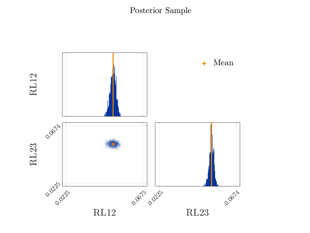
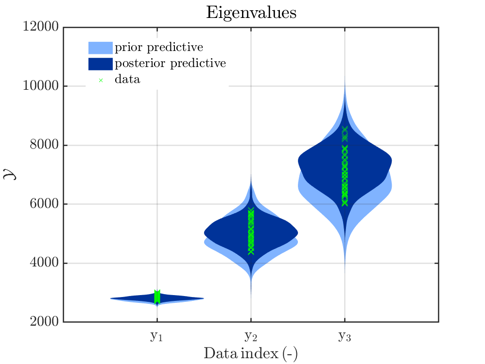
The posterior predictive eigenvalue distributions seem to be correct, but the updated parameter distributions are too narrow. If, using the updated parameter distributions, I regenerate the eigenvalue distributions, then they are too narrow and do not agree with those in the figure. It seems that UqLab adds something to the predictive posterior (eigenvalue) distributions. Could it be that the prior discrepancy was added to the posterior eigenvalue prediction?

I am almost sure the problem is in how I calculated the discrepancy model from the manuals - it is not clear to me how to do that. Someone can help me please?

I also assumed the discrepancy unknown (section 2.2.6.2 of the manual). However, the results are close to the ones described above.

Dear Irma Isnardi,

starting with an answer to the problem how the predictive posterior distributions is created by UQLab: For all derived sample pairs of values for RL!2 and RL23 the model output is computed and afterwards a sample for the discrepancy is added, using either the known fixed values for the variance in the different components in DiscrepancyOpts.Parameters or, if you use a unknown discrepancy following section 2.2.6.2, the posterior density sample will be computed from the sample value for the discrepancy/variance value accompanying the sample value for RL12 and RL23 as third components in the sample triple.
If you are interested in plots of the density of the model outputs without the added noise, you may use the function in the topic Further plot possibilities for results of Bayesian inversion (Suggestions and code example), at least if you are still using UQLab 1.4. I have not tested my function with UQlab V2.0 yet.

Here a remark: Since you have used 3 different discrepancy vales for the three output components of your model, you should maybe consider for each of your components a separate prior and posterior density for the discrepancy, i.e.instead of following section 2.2.6.2, you should follow the discussion an the end of section 2.3.4.2, with the modification that you will need define a marginal with three components and not only two.

If I understand correctly, you have an experiment that allows you to get observations belonging to different values for the model parameters that are samples for some controlled parameter uncertainty, and you want somehow reproduce this uncertainty by using UQLab to apply the Bayesian Theorem. If this correct, then I have bad news, since
this will not work, at least not directly. I have tried this myself in the past, and had to realize that even if in many books and literature is it claimed that one application of the Bayesian Theorem allows to extract information about some hidden parameter density generating the observations, this is not true, since one application of the Bayesian Theorem generates a posterior density containing the information on the single parameter value that created all observations since different measurements errors are considered, and not more.

For example, If one is considering a linear model, has derived a prior density for the parameter and a value for discrepancy and is dealing with observation y_1, y_2,....y_K then it holds for the posterior density following from the Bayesian Theorem, that one can get the same posterior density if one considers as observation K repetitions of the mean of y_1, y_2,....y_K.
Considering the general situation, see e.g. the derivation in Sections 1.2.2 and 1.2.3 of the manual, it holds that the model output \mathcal M(\mathbf{x}) for one paraemter value \mathbf{x} is considered as approximation of all observations, i.e. it is somehow assumed that the observations only differ because there were different values for the measurement errors between the different observations of the same value. Therefore, it holds in your computations that the density computed by UQLab represents the information that one has on the one parameter value x_{one} such that \mathcal M(\mathbf{x_{one}}) + noise creates all observations, see also my discussion in the following post Bayesian inversion : limit the correlation of posterior inputs - #4 by olaf.klein.
If you reduce the value for the discrepancy sufficiently you will get violin plots such that the many of the measured values are outside of the posterior “bubble”, i.e. the decrease in discrepancy will not increase the variation of the computed samples for the model parameter, as I believed for some time.
My solution to dealing with parameters values that are different for different observations, is to collect all observations belonging to one parameter value and to formulate the Bayesian problem on for these data. Doing this for all collections, you can perform one separate run of uq_createAnalysis for each of them, storing the different results. At the end, one could merge the sample array form the different ANALYSIS objects.

Hope that this still helps
Greetings
Olaf

2 Likes

Dear Olaf,
Thank you very much for your reply. I arrived at the same conclusion as you.
Do you know any references for this aspect of the Bayesian updating? As you wrote, many in the literature claimed that these types of applications are possible.
Kind regards,
Irma

Dear Irma,

I am not aware of any reference where this aspect of Bayesian updating is discussed.
According to my computations it holds that for a correct derivation for the formulae in Bayes’ theorem one has to to assume that the observation is as a noise modified output of the model for an input value being a sample of a random variable such that the density of this random variable is just the prior density. But, this is usually not pointed out since the formulae is not proved or the assumption is used in the proof without being formulated.

I should point out that there is a way to use Bayes’ theorem to deal with you problem, but then the the considered parameter “values” would not be the pairs of the two real numbers (RL12, RL23), but each parameter “value” would be a probability density on [0,\infty) \times [0,\infty). And the prior and the posterior density would be densities
on the set of these probability densities. Maybe there is a way to formulate an
approximation for the resulting formulae one can deal with, but I have no tried.

I would suggest instead to apply for each set of your observations that belongs according to your knowledge to the same input sample value Bayes’ theorem to extract information on this input value sample in the posterior density.
And considering all date sets and computing afterwards the average of these posterior densities (which represents to merge the sample for the parameter values) will somehow produce an approximation for the density representing the parameter uncertainty you want to identify, but it may be a bad one.
For example, if you have not enough data sets you may get a density that is quite small almost anywhere, but these are some disconnected regions with a high density. i.e. In view of samples, one would get a large region with almost no samples and some disconnected regions wherein there are many samples. Okay, even such a result may provide some useful information, but this is tricky to decide

Greetings
Olaf