Bayesian inference in UQLab: suggestions for improving the plot functions and the corresponding UQLab User Manual

[olaf.klein]

Bayesian inference in UQLab: suggestions for improving the plot functions
and the corresponding UQLab User Manual

Dear @paulremo, dear all

after starting to work with UQLab, performing some Bayesian inference computations, examining the program code of UQLab, and pointing out some errors in the code, I would like to suggest some changes in the graphic output and in the UQLab User Manual for Bayesian inference from a users point of view:

1. Legend “mean” / “mean prediction” in plots

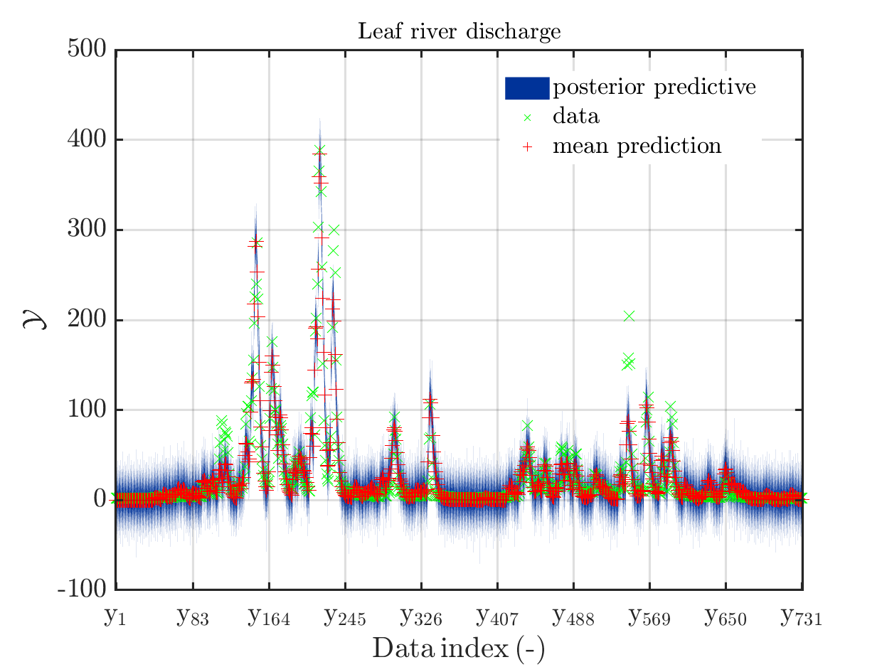
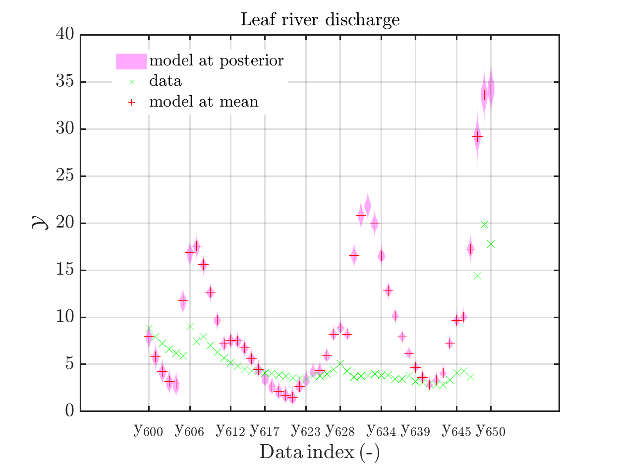
The current official version of uq_display_uq_inversion.m shows “mean” as legend for the red line in the plots for the predictive distribution to indicate
that the red line marks the value for the model output at the approximation for
\mathbb{E}(X|\mathcal{Y}) that is derived by computing the empirical mean of the samples for the model parameter generated from appropriate MCMC samples, at least according to my current understanding of the program code.

I must admit that I believed for some time that this “mean” is just the mean of the samples generating the shown predictive distribution.

In a preview version I got for uq_display_uq_inversion.m (thanks, Paul-Remo), the legend text “mean” is replaced by “mean prediction”, which is an improvement. But, I thins that also this notion could create confusion, since in many papers “mean prediction” corresponds to the mean of the derived predictions but here it is supposed to be the prediction derived by the evaluation the model at the mean of the samples for the model parameter generated from appropriate MCMC samples,
When I discussed results of my computations with a cooperation partner, being a UQ-expert, he asked me, which of these two interpretation of “mean prediction” is valid in my plots. Hence, it is proved that the notion “mean prediction” can create confusion and should therefore be replaced by a different notation, like e.g. “model(mean)” or “model@mean” or “model at mea” or …

---

2.) Inconsitent use of notion “point estimate”, fix of notations

I must admit that I am confused about the usage of “point estimate” in the manual,
in the program output and in the program code:

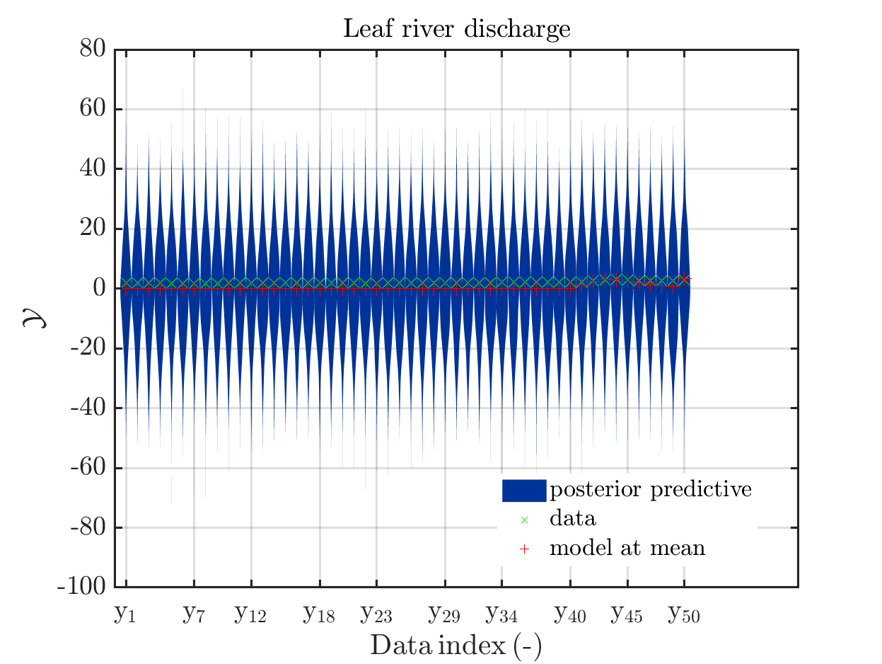
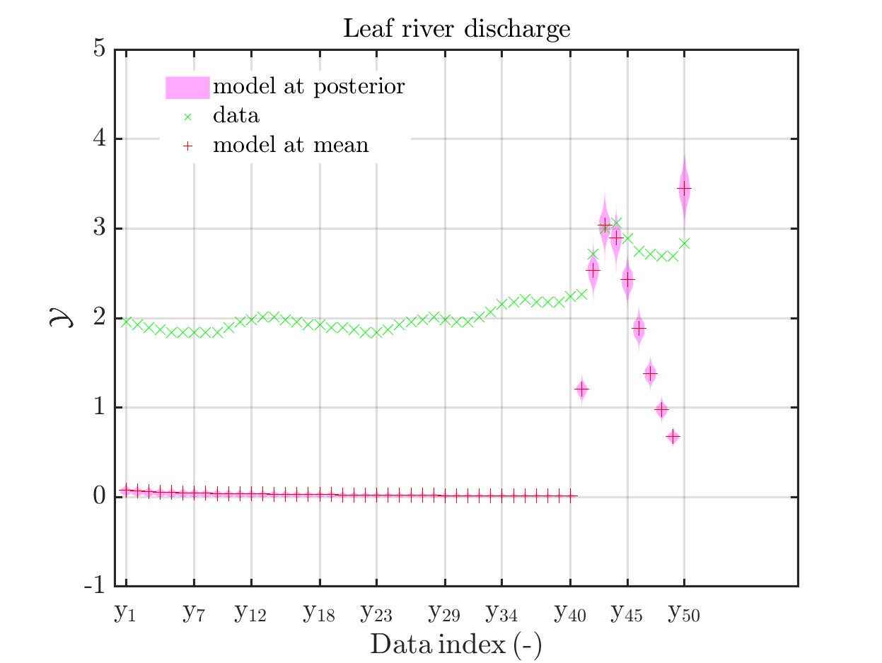
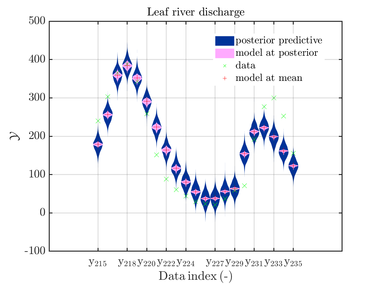
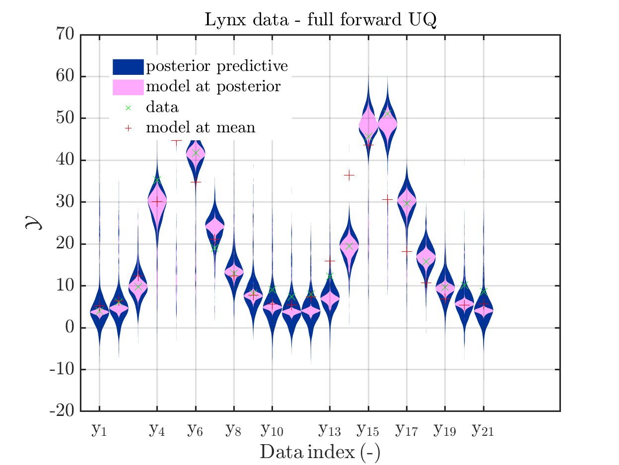
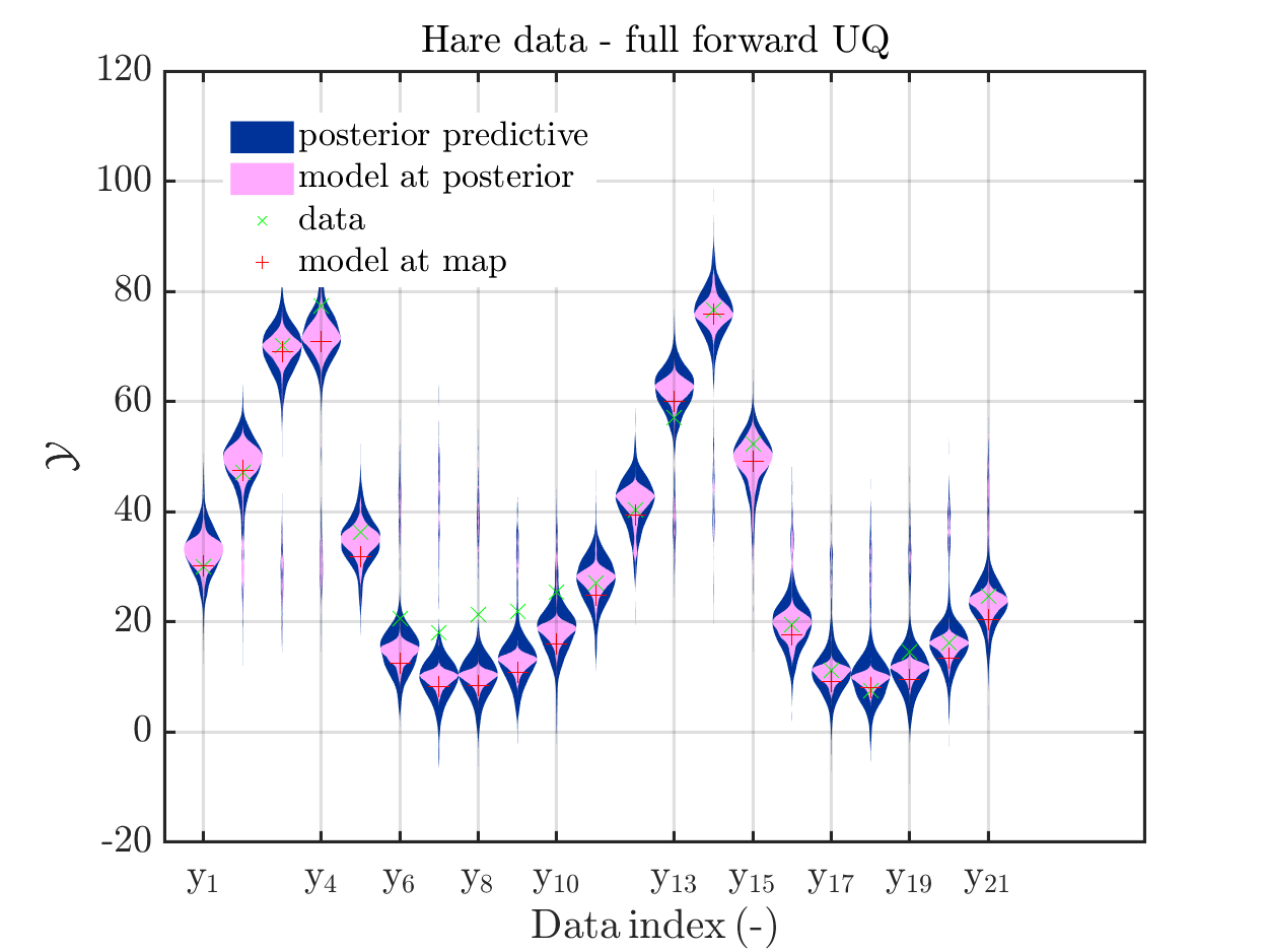
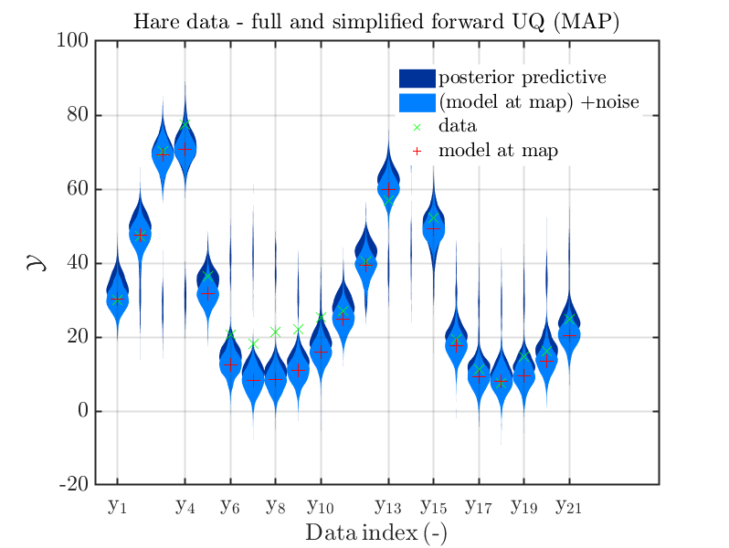
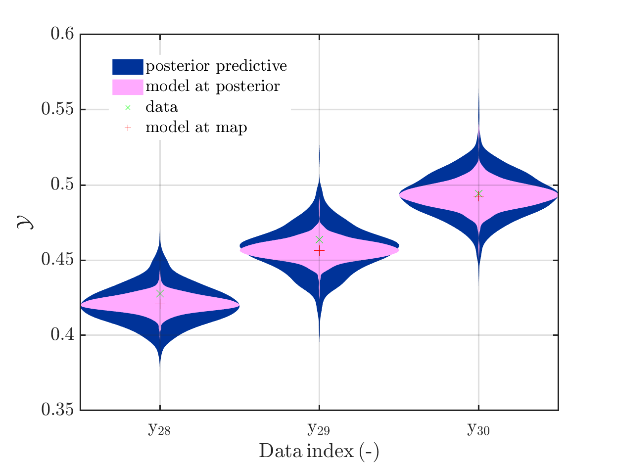
In view of the description of the plots in Fig 4(a), Fig 6(a), Fig 9(a) and the red mark in the plots, and what is shown in this plot according to the program code, “mean point estimate” (this notion is only used in these descriptions) seems to indicate the model output at the mean of the samples for the model parameter generated from appropriate MCMC samples.
But, in the description of Fig 4/6/9 it is also claimed that ``the empirical mean \mathbb{E} [X |\mathcal{Y}] estimated from the MCMC sample’’ is shown in Fig 4(a)/6(a)/9(a), which is not the case.
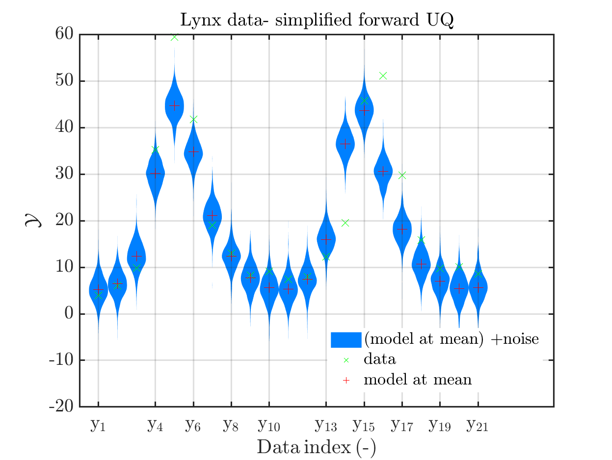
Hence, I wonder if maybe in both descriptions the mean of the samples for the model parameter generated from appropriate MCMC samples (that is shown Fig 4(b)/6(b)/9(b)) and the model output at this mean (that is shown Fig 4(a)/6(a)/9(a))
has been mixed up.

This would be compatible with an interpretation of " mean point estimate" in view of to the program output, other parts of the manual and the program code.

In the outputs of uq_print, see e.g. on the pages 21, 26, and 41, of the manual, it holds that there is a table entitled “Point estimate” and a row entitled “Mean”, providing the means of the samples for the model parameter and for the discrepancy generated from appropriate MCMC samples. Hence, it seems to be natural to denote this mean by “mean point estimate”.

Moreover, this interpretation seems to be compatible with the the discussion on emph{point estimator} on page 3 and the discussion near to equation (1.20).

Moreover, in view of the program code of uq_postProcessInversion, it holds that if the flag pointEstimate_flag is true, and the value of pointEstimate is “mean” the resulting value for module.Results.PostProc.PointEstimate.X is the mean of the samples.

I have not been able to find a general established interpretation for “mean point estimate” in my UQ books or by a Internet search .

I suggest to fix a notion for the mean of the samples for the model parameter
and for the model out[t at this mean in the UQLab User Manual for Bayesian inference and use it consistently.

To fix the notion, I suggest to add a new section 1.3.6:
To simplify my argumentation, I will use the notion therein in my text afterwards. following.

1.3.6: Quantities derived from results of a MCMC simulation

After performing a MCMC simulation, and a reduction of the derived sample due to
the burn-in and, if necessary, removing of bad chains (see Section 3.3), one can draw a set of samples from the remaining samples in the reaming MCMC chains. From these extracted samples one can compute a number of quantities.
In the following, we use the following notions to describe some them:

• mean point estimate:
  the empirical mean of the parameters values in the extracted samples, being an
  approximation for the posterior mean, i.e. for the empirical parameter mean \mathbb{E}[X | \mathcal{Y}] as in (1.20)

• model output at mean point estimate:
  output of the model if it is evaluated at the mean point estimate

• model(mean) :
  legend text used in plots indicating the model output at the mean point estimate

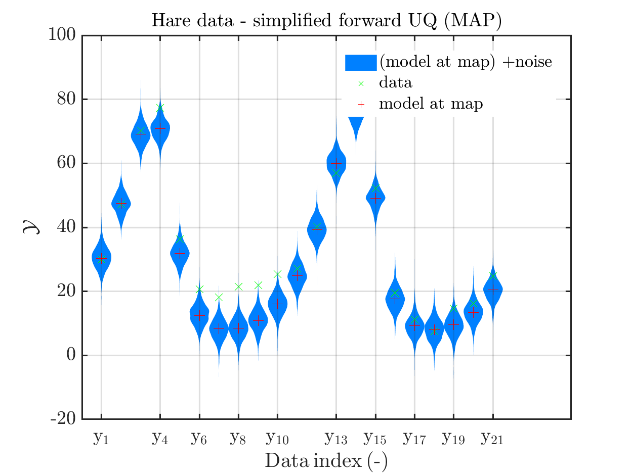
• MAP point estimat:
  set of parameters values in the extracted samples where the maximum of the posterior over all these samples is attained. This is an approximation of the
  posterior mode, a.k.a. the maximum a posteriori (MAP),

• model output at MAP point estimate:
  output of the model if it is evaluated at the MAP point estimate

• model(MAP):
  legend text used in plots indicating the model output at the MAP point estimate

The samples for the posterior sample points are derived form the samples extracted from the MCMC samples following the considerations in the end of Sections 1.2.5 and 1.2.6. [My suggestion for a new section 1.2.6 follows below in point 7.]

---

3) Suggetion to add references to descriptions of plot contents

I suggest to add to the description of the plots in Fig. 4, 6, and 9, a reference/ references to the description(s) of the contents of the plot that can be found in Section 1 (e.g. to the new Section 1.3.6 if you decide to follow my suggestion).
This would help thereader to find these information especially if she/he needs information on the plot contents to understand some unexpected results in the plots in her/his application, and had forgotten during the programing period the details of the content of section 1.

---

4) Inconsistency between plot and its description

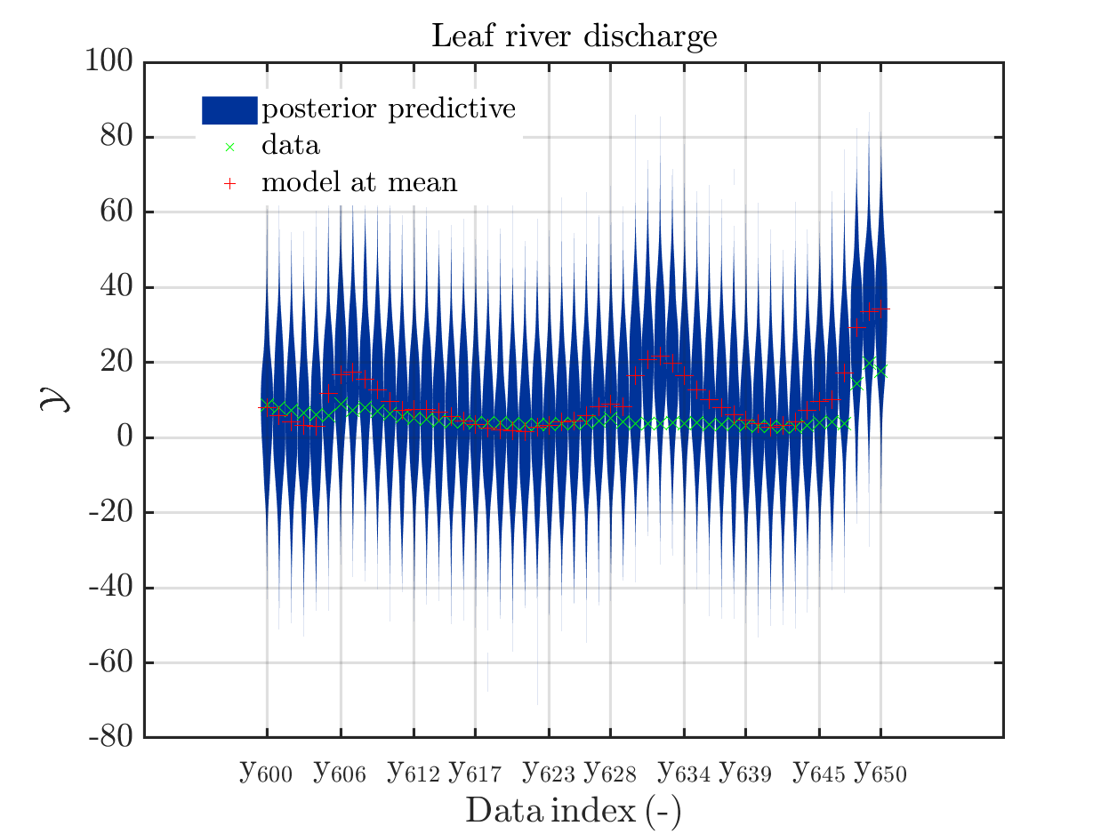
Page 23, Figure 4(a): In the current plot, there is no prior predictive distribution shown, but listed as content of the plot in its description.
Hence, I suggest to adapt either either the description or the plot.

---

5) Adding a legend to scatter plots

When dealing with scatter plots, it would be helpful if in
the plot there would be a legend indicating if
the mean point estimate or the MAP point estimate is marked.

---

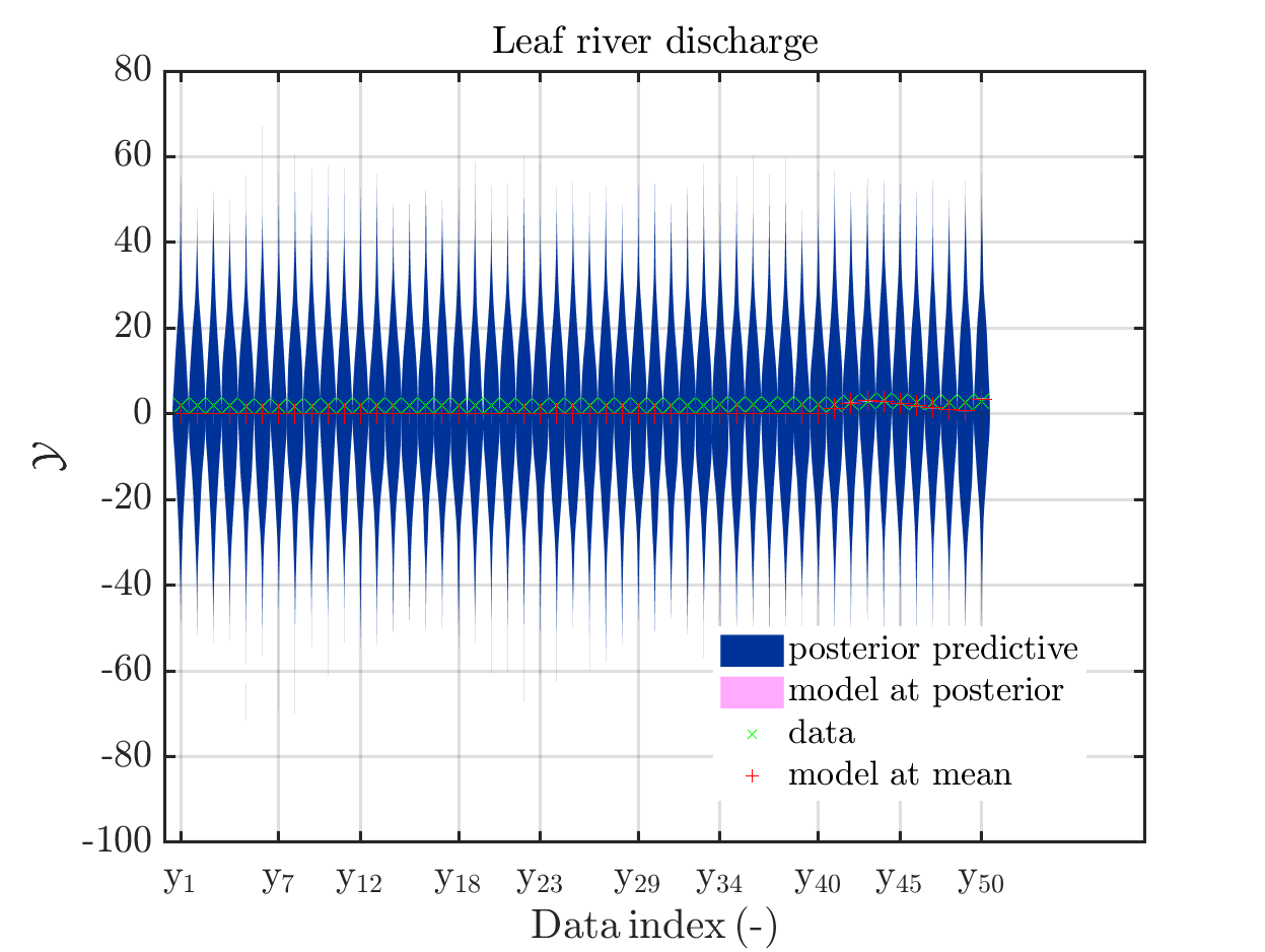
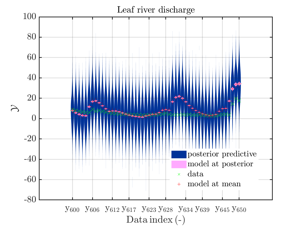
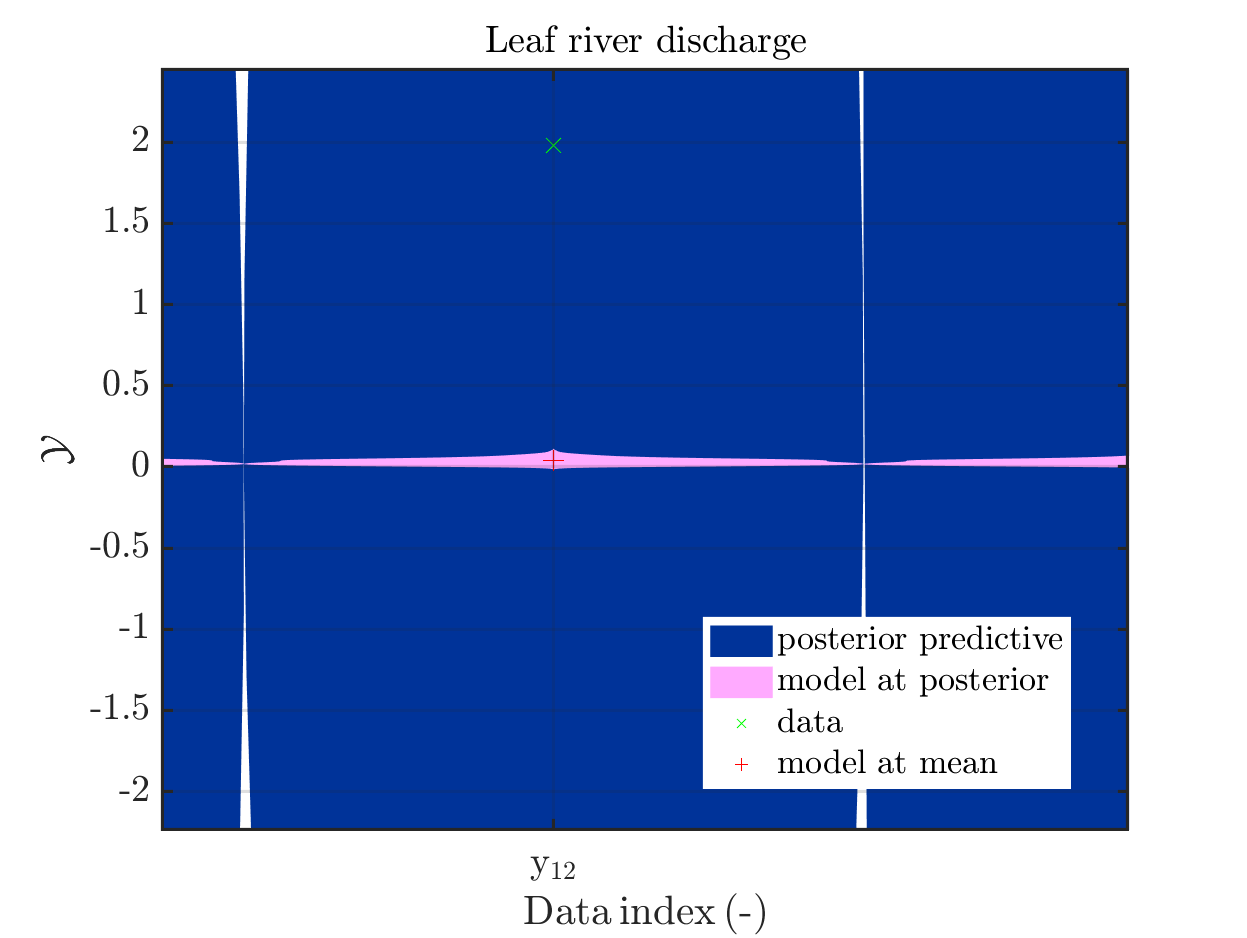
6) Emergency meassures if plot legend hides important parts of plot

When I prepared my Case study Example of Bayesian inference computation creating a model output at the mean of the parameter samples that is outside of the discrete posterior predictive support I had to repeat the derivation of the example since in some cases the legend in the plot for the posterior predictive distribution plot was hiding the marks for the model output at the mean of the sample.
Since hiding of important part of the plots may also occur if one is dealing with the result of a fixed application, it may be helpful if there would be the emergency possibility to use a new option to the call of uq_print to either change the position of the legend within the plot or to show the legend in a separate figure.

---

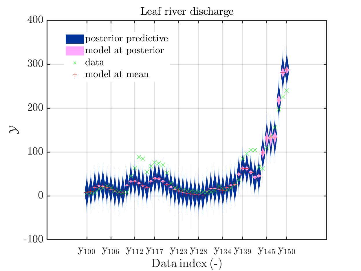
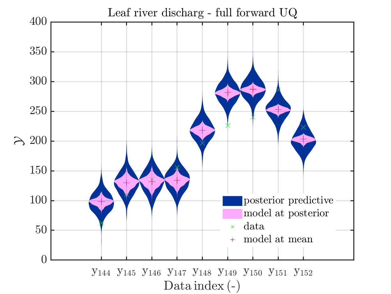
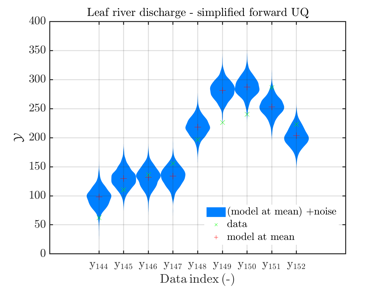
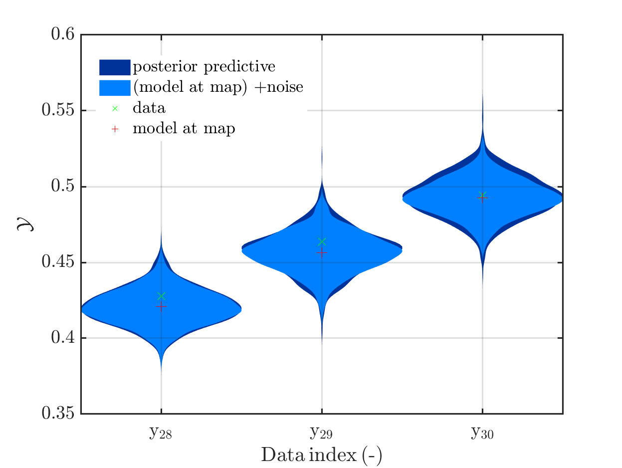
7) Formulation of Section 1.2.5 ``Model predeictions’’ only valid for a discrepancy with known parameters

I think that the current formulation of Section 1.2.5 ``Model predeictions’’ of
the manual is only valid for a discrepancy with known parameters, and does not
represent the calculations currently implemented in uq_postProcessInversion to derive a sample for the posterior predictive, if a discrepancy with unknown parameters is considered

For dealing with this situation, the following calculation is implemented:

Starting from samples x_i = \left( x_{i, \mathcal M}, x_{i,\varepsilon} \right) for \mathbf{x} = \left( \mathbf{x}_{\mathcal M}, \mathbf{x}_{\varepsilon} \right)
that were drawn according to \pi(\mathbf{x} | \mathcal Y), one evaluates \mathcal{M}(x_{i,\mathcal M}), and
draws independently samples from \mathcal{N}(\varepsilon|M(x_{i, \mathcal M}),x_{i,\varepsilon} ....) (I am not sure about the exact form that is possible for the matrix there) to derive samples for the posterior predictive.)

I suggest to change the title of of Section 1.2.5 to “Model predictions for discrepancies with known parameters” and to add a new section 1.2.6: *“Model predictions for discrepancies with unknown parameters”’’ dealing with this situation.

---

I hope that you like at least some of my suggestions.

Best regards
Olaf

[paulremo (Paul-Remo Wagner)]

Dear @olaf.klein

Thank you very much for your detailed review of the Bayesian module. I will have a look but I am sure that many of your suggestions will make it to the next live version!

[olaf.klein]

Dear Paul-Remo, dear all,

as an extension of my remarks above, I would like to present a modified version of the function plotSeriesPred.m from the UQLab File uq_display_uq_inversion.m (UQLab v.1.3+, i.e. the developer version derived from UQLab v.1.3. Thanks to @paulremo again.) in the file mod_UQLab_plotSeriesPred.m (9.3 KB)

New function in file mod_UQLab_plotSeriesPred.m

I modified the function plotSeriesPred.m to get access to further informations produced during the Bayesian inversion performed by the evaluation of uq_createAnalysis.

One point is to consider on one hand the variation of the posterior predictive samples, i.e. the sum of the model output at the samples and appropriate noise and on the other hand the variation of the model outputs at these samples only.

Moreover, one may need information to decided how to perform further computations using the results of the Bayesian inversion. Here one has to decide, if one should perform a forward UQ computation or if one can expect to derive similar results by performing a reduced forward UQ computation, i.e. by evaluating the model only at a point estimate for the parameters, like the mean of posterior density or the MAP value, and adding afterwards some noise values to this output value.

To decide this, I think that one should investigate to the results of the Bayesian inversion form a other point of view.: The resulting posteror predictive density is the density one one would get from the output of a (ful)l forward UQ computation for the considered model using the the density represented by the derived samples for the parameter values.
Moreover, by adding the discrepancy samples used for the computation of the posterori prediction samples to the model output either for the mean of the posterior density or MAP point estimate, one can compute the results corresponding to a reduced forward UQ computation.

If these densities are quite different, one can expect that also in other situations the results of a reduced forward UQ computation will not generated good approximations for the results for a (full) forward UQ computation. But, if the results are similar then I think that there is some chance/risk that the results of the reduced forward Uq computation allow to approximate the results for the full forward UQ computation. This can be good nesw, if one is only interested to compute this approximation. But, this can also be bad news, if the considered problem was planded to promote dealing with UQ considerations.

I think that this function may also be helpful for other users of UQLab.

To be able to use this function, one must use the files uq_display_uq_inversion.m, uq_initialize_uq_inversion.m, and uq_postProcessInversion.m provided by Paul-Remo in one of his posts to the topic Bayesian inference with multiple forward model with different numbers of provided measurements but with one common discrepancy model and parameter?)
The modified function in `mod_UQLab_plotSeriesPred.m’ has the following features;

1. The output for all plot types can be restricted to show only data points within a given index range.

2. The density of the model evaluations at the samples of the posterior density, i.e. the contents of myBayesianAnalysis.Results.PostProc.PostPredSample.Post,
   can be ploted, see the examples with 'model' as plot type parameter, i.e. as thrird parameter. .

3. The normal posterior predictive density plot can be combined with the density discussed in the last point. This allows to deiced if the variation shown for a data point contain mainly the variation due to the noise or if the value of the model also shows significant variations due to variation of the parameter values. This can be achieved by using 'postMod' as plot type parameter.

4. To check if the reduced forward UQ computations can be expected to generate relevant outputs, one can evaluate the model at the point estimate and add afterwards noise to the resulting value. This noise is just the difference between the values in myBayesianAnalysis.Results.PostProc.PostPredSample.PostPred
   and myBayesianAnalysis.Results.PostProc.PostPredSample.Post. This can be achieved by using 'Mod(PE)+noise' as plot type parameter.

5. One can combine the posteriori predictive density and the density discussed in the point before inte one plot by using 'postMod(PE)+noise' as plot type parameter. (This plots could be improved if there is any way to create a modification of uq_violinplot such that the generated plot would only contain the boundary of the density region.)

Example: Hydrological model calibration

To start to consider the examples for Hydrological model calibration at https://www.uqlab.com/inversion-hydrological-model further, one can use the following commands:

uq_Example_Inversion_03_Hydro 
uq_display(myBayesianAnalysis)

The posterior predictive density plot will look like

One can investigate the approximation of the Leaf river discharge either by using the zoom in feature in the matlab grafic window or by the commands

mod_UQLab_plotSeriesPred(mySamples,myData,'post',myPointEstimate,0,50)
title('Leaf river discharge');

mod_UQLab_plotSeriesPred(mySamples,myData,'post',myPointEstimate,50,100)
title('Leaf river discharge');

mod_UQLab_plotSeriesPred(mySamples,myData,'post',myPointEstimate,100,150)
title('Leaf river discharge');

mod_UQLab_plotSeriesPred(mySamples,myData,'post',myPointEstimate,150,200)
title('Leaf river discharge');

mod_UQLab_plotSeriesPred(mySamples,myData,'post',myPointEstimate,200,250)
title('Leaf river discharge');

mod_UQLab_plotSeriesPred(mySamples,myData,'post',myPointEstimate,250,300)
title('Leaf river discharge');

mod_UQLab_plotSeriesPred(mySamples,myData,'post',myPointEstimate,300,350)
title('Leaf river discharge');

mod_UQLab_plotSeriesPred(mySamples,myData,'post',myPointEstimate,350,400)
title('Leaf river discharge');

mod_UQLab_plotSeriesPred(mySamples,myData,'post',myPointEstimate,400,450)
title('Leaf river discharge');

mod_UQLab_plotSeriesPred(mySamples,myData,'post',myPointEstimate,450,500)
title('Leaf river discharge');

mod_UQLab_plotSeriesPred(mySamples,myData,'post',myPointEstimate,500,550)
title('Leaf river discharge');
    
mod_UQLab_plotSeriesPred(mySamples,myData,'post',myPointEstimate,550,600)
title('Leaf river discharge');
  
mod_UQLab_plotSeriesPred(mySamples,myData,'post',myPointEstimate,600,650)
title('Leaf river discharge');

mod_UQLab_plotSeriesPred(mySamples,myData,'post',myPointEstimate,650,700)
title('Leaf river discharge');
 
mod_UQLab_plotSeriesPred(mySamples,myData,'post',myPointEstimate,700,750)
title('Leaf river discharge');

These commands generate get a series of 13 plots showing the evolution in more detail,
see e.g.

Considering for the same data ranges as in these four plots the output of the models at the samples for the parameters for the HYMOD watershed model one can get corresponding plots by the commands

mod_UQLab_plotSeriesPred(mySamples,myData,'model',myPointEstimate,1,50)
title('Leaf river discharge');

mod_UQLab_plotSeriesPred(mySamples,myData,'model',myPointEstimate,100,150)
title('Leaf river discharge');
   
   
mod_UQLab_plotSeriesPred(mySamples,myData,'model',myPointEstimate,200,250)
title('Leaf river discharge');
   
mod_UQLab_plotSeriesPred(mySamples,myData,'model',myPointEstimate,600,650)
title('Leaf river discharge');

Comparing the resulting plots
with those above showing the posterior predictive density, one observes that the variation of the posterior predictive values is much larger as the variation of the model outputs.

Creating the combined plots by the commands

mod_UQLab_plotSeriesPred(mySamples,myData,'postModel',myPointEstimate,1,50)
title('Leaf river discharge');

mod_UQLab_plotSeriesPred(mySamples,myData,'postModel',myPointEstimate,100,150)
title('Leaf river discharge');
      
mod_UQLab_plotSeriesPred(mySamples,myData,'postModel',myPointEstimate,200,250)
title('Leaf river discharge');
   
mod_UQLab_plotSeriesPred(mySamples,myData,'postModel',myPointEstimate,600,650)
title('Leaf river discharge');

one gets

In some of the plots, one can only see he density plot for the model output variation by using the zoom in feature of the matlab graficwindow, leading for example to

Now, two index ranges are considered such that the size of the model output variation compared
to the variation of the posterior predictive is larger as for other index ranges. To compare for those ranges the posterior predictive distribution, which interpreted as the output of a (full) forward UQ using the computed posteriori density, with the result of the simplified forward UQ, i.e. adding appropriate noise values to the model output at the mean point estimate, one can create these plots with the commands

mod_UQLab_plotSeriesPred(mySamples,myData,'postModel',myPointEstimate,144,152)
title('Leaf river discharg - full forward UQ');

mod_UQLab_plotSeriesPred(mySamples,myData,'Mod(PE)+noise',myPointEstimate,144,152)
title('Leaf river discharge - simplified forward UQ');

mod_UQLab_plotSeriesPred(mySamples,myData,'postModel',myPointEstimate,215,235)
title('Leaf river discharge - full forward UQ');

mod_UQLab_plotSeriesPred(mySamples,myData,'Mod(PE)+noise',myPointEstimate,215,235)
title('Leaf river discharge - simplified forward UQ');

In view of the correspondig plots,



one may conclude that it may be sufficient to perform a simplified forward UQ to derive furter predictions for the Leaf river discharge, or one may switch between the simplified forward UQ and the full forward UQ depending on the computed value for of the discarge.

Predator-prey model calibration

Considering the predator-prey model calibration as in https://www.uqlab.com/inversion-predator-prey one can use the commands

uq_Example_Inversion_04_PredPrey

% Extract data from myBayesianAnalysis
myData = myBayesianAnalysis.Data
DataTest = myBayesianAnalysis.Data
mySample = rmfield(myBayesianAnalysis.Results.PostProc.PriorPredSample,'Prior');
mySample(1).PostPred= myBayesianAnalysis.Results.PostProc.PostPredSample(1).PostPred
mySample(2).PostPred= myBayesianAnalysis.Results.PostProc.PostPredSample(2).PostPred
mySample(1).Post= myBayesianAnalysis.Results.PostProc.PostPredSample(1).Post
mySample(2).Post= myBayesianAnalysis.Results.PostProc.PostPredSample(2).Post
myPointEstimate = myBayesianAnalysis.Results.PostProc.PointEstimate.ForwardRun

mod_UQLab_plotSeriesPred(mySample(1),myData(1),'postModel',...
    myPointEstimate);
title('Hare data - full forward UQ')

mod_UQLab_plotSeriesPred(mySample(1),myData(1),'Mod(PE)+noise',...
    myPointEstimate)
title('Hare data - simplified forward UQ')

mod_UQLab_plotSeriesPred(mySample(2),myData(2),'postModel',...
    myPointEstimate);
title('Lynx data - full forward UQ')

mod_UQLab_plotSeriesPred(mySample(2),myData(2),'Mod(PE)+noise',...
    myPointEstimate)
title('Lynx data- simplified forward UQ')

These commands produce for the hare data a plot showing the combination of the posterior predictive distribution, which can be interpreted as the result of a full forwards UQ computation of the densities derived by the result of the performed inverse UQ and of the model output variation showing the result of the simpliefed forward UQ using the model outpt at the mean of posterori density, see

Moreover, a similar pair of plots is created for the lynx data, see

Hence, here one can observe that quite often the variations of the model output are of the same order as the variations of posteriori predictive distribution. Moreover conparing the results for the hare data at the indizes 3,4, 10, 11, 12, 14, 15, 19, 20, 21 and for the lynx data at the indizes 5, 13, 14, 16, 17 it is obvious that the results one can get from the simplified forwards UQ computation using the model output at the mean is not appropriate to approximate the results of the full forwars UQ computation.

To get plots such that the mode evolutation at the mean of the posteriori density is replaced by the model evolution at the MAP point estimate, one has to perfrom the following commands:

uq_postProcessInversion(myBayesianAnalysis,...
                        'badChains', badChainsIndex,...
                        'prior', 1000,...
                        'priorPredictive', 1000,...
                        'posteriorPredictive', 1000,...
            'pointEstimate','MAP');
                    
% Update sample value to keep consistency   
myMapData = myBayesianAnalysis.Data

myMapSample = rmfield(myBayesianAnalysis.Results.PostProc.PriorPredSample,'Prior');
myMapSample(1).PostPred= myBayesianAnalysis.Results.PostProc.PostPredSample(1).PostPred
myMapSample(2).PostPred= myBayesianAnalysis.Results.PostProc.PostPredSample(2).PostPred
myMapSample(1).Post= myBayesianAnalysis.Results.PostProc.PostPredSample(1).Post
myMapSample(2).Post= myBayesianAnalysis.Results.PostProc.PostPredSample(2).Post
myMapPointEstimate = myBayesianAnalysis.Results.PostProc.PointEstimate.ForwardRun       

% plot posteriori predictive density and model output density for 
%  hare data 10,...,20 
mod_UQLab_plotSeriesPred(myMapSample(1),myMapData(1),'postModel',...
    myMapPointEstimate);
title('Hare data - full forward UQ')

mod_UQLab_plotSeriesPred(myMapSample(1),myMapData(1),'Mod(PE)+noise',...
    myMapPointEstimate)
title('Hare data - simplified forward UQ (MAP)')

mod_UQLab_plotSeriesPred(myMapSample(1),myMapData(1),'postMod(PE)+noise',...
    myMapPointEstimate) 
title('Hare data - full and simplified forward UQ (MAP)')

mod_UQLab_plotSeriesPred(myMapSample(2),myMapData(2),'postModel',...
    myMapPointEstimate);
title('Lynx data - full forward UQ')

mod_UQLab_plotSeriesPred(myMapSample(2),myMapData(2),'Mod(PE)+noise',...
    myMapPointEstimate)
title('Lynx data- simplified forward UQ (MAP)')

mod_UQLab_plotSeriesPred(myMapSample(2),myMapData(2),'postMod(PE)+noise',...
    myMapPointEstimate)
title('Lynx data- full and simplified forward UQ (MAP)')

Considering the resulting plots for the hara data



(the last plot shows the density of the posteriori predictive combined with the density for
the simplified UQ computation) and the plots for the lynx data

we see that changing to the MAP estimate as improved the result of the simplified forward UQ compuations, but considering the hare data at the indizies 1,2,5,10,11,12,21, the lynx data at the indix 4, and the missing rare events in the simplifed forward Uq results yiels that changing to the MAP point estimate has improved the approximation but the results of the simplified forward UQ are still not sufficient to suggest to use the simplified forward UQ for further considerations.

My model

It is my plan, to solve an Bayesian inference problem to identify the model parameters and their uncertainties and to use afterwards these information, i.e. the representation by the samples in myBayesianAnalysis.Results.PostProc.PostSample (see also the corresponding post of Paul-Remo) to perform forwards UQ computations. After using UQLab/ uq_createAnalysis, I get with my new plot function that for most data points the variation of the model output is much smaller then the variation of posterior predictive density. For some data points these variations are of the same order, see

But also for these points it holds that posterori preditive density, i.e. the results of the full forward UQ,
and the result of adding noise to the model output at the MAP estimate for paraemter values representing the result a simplified forward UQ, are almost identical, see

Hence, I fear that considering this problem further may not allow to show that one should use full forward UQ and not only the simplified forward UQ.Hence, this problem may not be a good example to convince other people that the computation related to UQ are quite important.

Greetings
Olaf

[paulremo (Paul-Remo Wagner)]

Many of the feature requests mentioned in this topic have been adressed in the previous UQLab release (v1.4). For other features that have not been adressed, there exists a follow-up topic, which is why I am closing this one now.