As you are well-aware, it seems appealing to apply meta-models such as Kriging, PCE, PCK, and so on in finding reliable alternative formulations of original nonlinear FEM problems. UQLab with its capability of using a vast variety of meta-models seems a brilliant tool for this purpose.
I tried to find the equation such as (1.27) in the Kriging manual. My problem has 4 random variables. I set different options as follows:
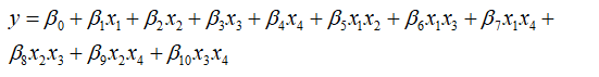
Also, I examine the other option (Degree=1, ‘polynomial’) but the size of beta is constant, it is equal to 10. I am confusing how to find the formula as below:
In a sentence, I want to guide me on how to find a reliable alternative metamodel-based equation?
I really appreciate your sustainable guidance. Accordingly, I want to thank Prof. @ bsudret
I tried to reproduce your problem but I couldn’t. Here are a couple of remarks based on the description of your problem:
The configuration option for the Kriging trend is typically set via MetaOpts.Trend and notMetaOpts.Kriging.Trend, unless you are creating a custom Kriging model, in which none of the Kriging parameters are estimated.
If you intend to use MetaOpts.Trend.Type= 'quadratic' trend type, then MetaOpts.Trend.Degree wouldn’t be relevant because quadratic means polynomial degree 2. It won’t make much sense to have a quadratic trend with a degree other than 2. See, for instance, Table 2 page 25 of the Kriging User Manual.
With degree 2 you should get 15 beta coefficients because the trend equation for 4-parameter model would be (I explicitly write each term below. Note: I don’t keep the ordering of the coefficients as in UQLab here, but you should get the idea):
If you set the trend type to polynomial and the degree to 1, you should get five beta coefficients. So I am not sure why you get only one (see below).
Finally, if you use built-in 'polynomial' trend type, you cannot exclude the term x_1^2, x_2^2, x_3^2, and x_4^2 from the trend equation. Creating a trend function you wrote should be possible using a custom trend, but I just need to confirm that you explicitly don’t want those terms.
BTW, we could not speak about specific values of beta because it will depend on your particular case, but we can verify its size nevertheless.
As a verification example, I created two Kriging models for the 4-dimensional Rosenbrock function, one with a quadratic trend and the other with a polynomial of degree 1.
Thank you so much for your comprehensive explanations and appreciate the time you spent for me.
I try to find the trend equation for PCE and PCK. Is it possible to get a trend equation with PCE and PCK?
I examined one example with PCE and saw this warning:
Warning: The option “Trend” is not a valid option for Model 2, it will not be used.
I added just this option in PCE example:
MetaOpts.Trend.Type = ‘quadratic’;
Does it need to have more options?
I want to be sure that the PCE and PCK metamodels have this ability to provide the trend equation such as Kriging or no? In a sentence, Is it possible to have a surrogate formulation by PCK and PCE or not? How?
In UQLab, the notion of trend in a metamodel is specific to and therefore only applicable for Kriging and PCK metamodels. With PCK, PCE is used as the trend function in a Kriging model; that’s why you can still find beta coefficients for the trend function there.
Seen as a black box, all the metamodels in UQLab do the same thing: predict the output based on a given input. However, the underlying formulations of these metamodels may fundamentally be different (for example, PCE vs. Kriging). There is, for sure, a distinct surrogate formulation for each metamodel; the options in the corresponding UQLab metamodel are relevant only to that formulation.
I’d like to encourage you to have a look at least the theory section of each metamodel user manual (at least the ones you’re interested in) to see how they differ (or similar, depending on one’s perspective) to each other.
I read the user manual for PCK, PCE and Kriging. The trend code is attached for PCK and Kriging with rosenbrock function. I get the constant beta size for kriging metamodel equal to 15.
In contrast, in PCK, the beta size is achieved a fluctuation value, for instance in one run get 26 in another get 41, …
Could you help me to find my mistake?
As I mentioned before, in PC-Kriging, the trend term in the Kriging formulation is a PCE. This PCE in turn is determined by the LARS algorithm (this is the default; See PCE User Manual Section 1.5.2 for details on the algorithm). The coefficients of the trend term obtained by this iterative algorithm depend on the particular experimental design points. If the design points change, there’s a good chance that the coefficients differ; not only their values but the whole structure of the PC expansion as well.
Now in your code, the specification of the experimental design is this line:
MetaOpts.ExpDesign.NSamples = 50;
Using this specification, UQLab will automatically (and internally) generate 50 experimental design points based on myModel (the full computational model) and myInput (the probabilistic input model) you created before. Every time you call uq_createModel for PCK, a new experimental design is generated. So it is normal that you get a different number of coefficients because the LARS algorithm operates on a different set of points. In the convential Kriging model, you set the trend to be quadratic, and because there’s only one form of quadratic in UQLab, the trend always has 15 coefficients.
If you want to get the same results from each time you call uq_createModel for PCK, there are two ways:
Set the random seed number before you call uq_createModel. This will ensure that the same experimental design points will be the same every time uq_createModel is called.
Generate the experimental design points separately and use the same design to create the PCK model. You can do this by specifying a pre-generated experimental design to MetaOpts.ExpDesign.X and MetaOpts.ExpDesign.Y configuration options, instead of specifying MetaOpts.Input and MetaOpts.ExpDesign.NSamples.
Also note that the option you set on Line 32: MetaOpts.Trend.Type = 'quadratic'; is irrelevant for a PCK model because the trend is not quadratic (as defined in the Kriging manual) but a PCE.
This, as you notice, won’t disrupt the calculation but you should be aware that the resulting trend is not quadratic in the PCK model as set by the option.
Because PCK uses both PCE and Kriging, it is important to understand for each method the underlying formulation, algorithms involved, as well as the default of the relevant options used in UQLab.
I’m a bit curious though, what is it that you’re trying to do? Maybe you can tell a bit about the big picture of your original question.
I really appreciate your detailed answer.
My main purpose is to “Develop Explicit metamodel-based Formulation using UQLab”.
If I choose the Kriging metamodel, I have a specific beta-size vector to develop an explicit formulation.
In contrast, based on your fruitful discussion on the PCE-based trend of PCK approach using LAR method, I face fluctuating beta-size vector if I use different seed numbers.
I was wondering how I can develop a PCK-based explicit formulation with respect to the mentioned condition of having different “Number of Polynomials” in each run. Besides, if I set a constant seed number and achieving constant beta-size vector, there is no guarantee in the optimum seed number due to different LOO errors which is derived from different seed numbers.
Could you please elaborate what do you mean by explicit? Is the metamodel in UQLab not explicit or do you want to get the formula of a metamodel in UQLab? And are you focusing just on the trend function (because a Kriging predictor is more than just the trend)? In the title you mentioned “alternative metamodel-based formula”, what does it mean?
Also, I am not sure I understand what you mean by optimum seed number. Are you trying to get the best metamodel in perhaps somewhat “absolute” sense?
If you simply generate one realization of experimental design, you base your metamodel on that realization. With different realizations, the LOO errors would indeed differ from one realization to another. The rule of thumb is the larger the size of the experimental design, the fluctuation will be smaller. If you’re comparing different metamodels, it might be a good idea to keep the same experimental design for comparison.
Unless you cover every single points in the design space, indeed there is no guarantee that one metamodel is optimum for every realization; this is of course unrealistic for high-dimensional problem involving an expensive computational model. In practice, we build a metamodel because the alternative (evaluating the model directly) for UQ analyses is more expensive.