Introduction
Uncertainty quantification (UQ) has become a hot topic in virtually all domains of applied sciences and engineering in the last decade. In the research community, this relatively new field lies at the boundary of applied mathematics, statistics, and computational engineering sciences. In the last few years, not only the number of scientific publications in this area has blown up, but also new scientific journals[1] devoted to this topic have emerged. In parallel, several books, mostly with a high-level mathematical profile, have been published. In this respect, it is rather difficult for beginners to find their way. Even the Wikipedia page on uncertainty quantification rapidly gets into computational details and methods without mentioning “the big picture” first.
In this post, I would like to introduce UQ from a pragmatic approach. As such, it is intended for engineers and scientists who have developed a model to understand a phenomenon, design a system, make some predictions, etc. and are now confronted with questions like:
- How do uncertainties affect the predictions of my model? How to provide error estimates/confidence bounds on my results?
- What are the important parameters that drive the model predictions and/or their uncertainty?
- What combinations of parameters lead to extreme/non-acceptable behavior/performance? How likely are these extreme events?
- How to best calibrate my model from experimental data while accounting for uncertainties?
Figure 1 provides a general scheme that can be used to identify the key ingredients of any uncertainty quantification problem.
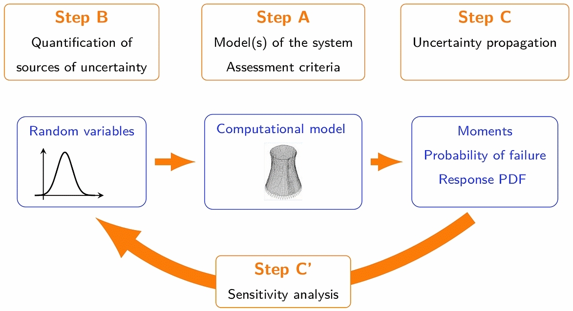
Figure 1: General scheme for posing uncertainty quantification problems (From Ref.1)
Computational model (Step A)
Whatever your discipline, you are probably familiar with computational models that represent some real phenomenon through a set of governing principles or equations. These are in turn solved either analytically or, in most practical cases, computationally by a dedicated solver. Examples include finite element models of structures in civil and mechanical engineering, hydraulic flood models and dissemination of pollutants in environmental engineering, circuits and power grid simulators in electrical engineering, chemical kinetics, weather forecast and climate change models, disease-spreading models in epidemiology, real business cycle models in economics, actuarial models for insurance, etc.
Across these fields, the nature of the governing equations can be very different. However, after proper implementation of a solver, the computational model can be seen as a black-box function that predicts quantities of interest as a function of input parameters[2]. For the sake of simplicity, we consider here that inputs are gathered into a vector \mathbf{x} of dimension d. The model is denoted by \mathcal{M} and allows us to compute a vector of quantities of interest \mathbf{y} = \mathcal{M}(\mathbf{x}).
… In practice
“Black-box” means that we only have access to runs of the computational model for specific values of the inputs. The associated uncertainty propagation methods are called non intrusive since they will not require any modification nor knowledge about the nature of your existing computational model. Of course, a UQ analysis will require repeated runs of the latter, so some form of automated batch execution for different sets of input parameters is to be expected!
Sources of uncertainties (Step B)
In standard applications, the computational model \mathcal{M} is deterministic: if you run it twice with the exact same input vector, you get the exact same output up to machine precision. However, you may not know exactly what input values to use to properly represent your real system/phenomenon. That’s where the UQ analysis start: how to identify and represent your sources of uncertainty?
Two main types of uncertainties are encountered in practice:
- you don’t know exactly the value of a parameter: you may have a best guess and possibly lower and upper bounds. This is called epistemic uncertainty: there is a “true” value, but you don’t know it, so you want to represent your lack of knowledge.
- Observations/measurements show that there is natural variability in the possible values of a parameter. This is called aleatory uncertainty.
The most common way to represent these two types of uncertainties is to use probability theory[3]: Each parameter is considered a random variable, for which a probability distribution is selected based on available information, expert knowledge, statistical analysis or a combination thereof (for instance, using Bayesian statistics).
… In practice
For each input parameter, you can start by defining:
- reasonable bounds, in the case of epistemic uncertainty. This can also be done in the format “best estimate value \pm xx%”. A uniform distribution is then an appropriate choice to represent the underlying uncertainty.
- or a distribution in the case of aleatory uncertainty. If you have data, applying standard statistical inference allows you to fit “the best” distribution. Even if there is no data, expert knowledge and literature in your field shall help you choose the right type of distribution. In most cases, the well-known Gaussian distribution is not a good choice!
- The question of statistical dependence between parameters need also to be addressed at this stage. Are there reasons to think that some parameters are correlated? If yes, this must be accounted for. A standard approach is to use a copula function to couple the marginal distributions of the input variables into a joint random vector.
Uncertainty propagation (Step C) and sensitivity analysis (Step C’)
Once (and only once) the model has been clearly described through its inputs and outputs, and a choice of probability distributions has been made for the inputs, one can proceed with uncertainty propagation to quantify the statistical properties of the output quantities \mathbf{y} caused by the uncertainty in the input parameters \mathbf{x}.
Depending on your problem, different statistics of \mathbf{y} may be of interest:
- the mean, standard deviation and other higher-order statistical moments
- the probability density function (PDF), to check if it is uni- (resp. multi)-modal, skewed, etc.
- the tail of the PDF, more precisely the probability of exceedance of a threshold
- the important input parameters, i.e. the ones which contribute most significantly to the response variability
- etc.
Monte Carlo simulation is a general technique for solving all these problems: first, you sample realizations of the input parameters using a random number generator. Then, for each sample, you run your computational model, and you collect the resulting realizations of the response. Using proper statistical estimators, you can, in theory, compute all the above-listed quantities. Monte Carlo simulation is however known to converge very slowly. You would typically need \mathcal{O}(100-1000) realizations when you are only interested in the second-order moments, whereas \mathcal{O}(10^5-10^7) is more common when dealing with small probabilities of exceedance or global sensitivity indices.
If your computational model is an analytical function or a simple computer code that runs in no time, you may afford this big number of realizations and it can be a good start. However, if you handle realistic high-fidelity computational models, you can most probably afford only \mathcal{O}(10-100) runs in a reasonable time. In this case, it is suitable to construct a surrogate model from this limited information, that is further used for the purpose of UQ. Popular surrogate models include polynomial chaos expansions, Gaussian processes (a.k.a. Kriging), neural networks, and support vector machines (SVM). You can find a concise introduction to these techniques here Refs.2,3,4.
… In practice
- Always start by properly defining the goals of your UQ study. If you are interested in small probabilities or in global sensitivity indices, completely different methods shall be used.
- Surrogate models are just a means to efficiently solve problems that would take forever to solve otherwise using Monte Carlo simulation. They are not UQ methods per se! In fact, surrogate models are also used for optimization, pattern recognition, weather forecasts, among others.
- However, it is well-known that (sparse) polynomial chaos expansions are a good technique to further compute moments and sensitivity indices, whereas Kriging and SVM combined with active learning techniques are suitable to compute extremely small probabilities.
And now, where to start?
If the keywords dropped in the previous paragraphs have rung a bell, you may already try to formulate your UQ problem following the rationale presented above. Then you probably want to have a look at a software package, install it, and run examples which are similar to your problem. We suggest the use of our software UQLab, because it has been designed to be extremely easy to handle for beginners that have only a basic knowledge of MATLAB. Other well-established software and packages in different languages are listed here.
… In practice
In most cases, the methods and tools required to solve your UQ problem already exist! There is generally no point in writing your own UQ routines from scratch since many optimized packages in virtually all languages are available. See this list for more info on some of the
available software!
In contrast, setting up the UQ problem by properly defining your goals, choosing the appropriate computational model, the probabilistic representation of its inputs (based on your current level of information and amount of data) and the relevant method for uncertainty propagation may require some time. Don’t hesitate to ask questions on this forum to get help!
References
- B. Sudret, Uncertainty propagation and sensitivity analysis in mechanical models - Contributions to structural reliability and stochastic spectral methods, Habilitation à diriger des recherches, Université Blaise Pascal, Clermont-Ferrand, France (229 pages), 2007.
- Marelli, S. and Sudret, B. UQLab user manual - Polynomial chaos expansions, Report UQLab-V1.2-104, Chair of Risk, Safety and Uncertainty Quantification, ETH Zurich, 2019.
- Lataniotis, C., Marelli, S. and Sudret, B. UQLab user manual - Kriging (Gaussian process modelling), Report UQLab-V1.2-105, Chair of Risk, Safety and Uncertainty Quantification, ETH Zurich, 2019.
- Moustapha, M., Lataniotis, C., Marelli, S. and Sudret, B. UQLab user manual - Support vector machines for regression, Report UQLab-V1.2-111, Chair of Risk, Safety and Uncertainty Quantification, ETH Zurich, 2019.
Back to the Chair’s Blog index
Notes
International Journal for Uncertainty Quantification, SIAM/ASA Journal of Uncertainty Quantification, ASCE-ASME Journal of Risk and Uncertainty in Engineering Systems ↩︎
In practice, each parameter could not only be a scalar but a time-series, a spatially-varying map, etc. ↩︎
Non-probabilistic representations using intervals, fuzzy sets, probability boxes, etc. are also used to represent epistemic uncertainties. It, however, raises computational issues when it comes to their propagation. See an overview in R. Schöbi, Surrogate models for uncertainty quantification in the context of imprecise probability modelling, 2017. ↩︎
 !
!