I am trying to do an probabilitic analysis based on Random Fields, on a finite element model, via UQLink. My aim is to set a PCE to surrogate the model’s response to this random Field.
Consider I have one input (say Young’s modulus), and my stochastic mesh corresponding to the random field is 10x10. I have a (continuous) correlation function, which describs the dependance between two elements, based on the distance between them (say \rho (x,x')).
I create samples of my Random Field with the EOLE method, and I am able to get the model’s response for those samples.
I have then a theorical problem with the creation of a PCE.
I’d like to set a PCE with the option Experimental Data, since some samples are already computed.
As specified in the UQlab User Manual, the implementation of the inputs is required in the PCE module. I am not sure which input I should specify.
On the one hand my theorical input is the underlying distribution of the Young’s Modulus, which is only one input.
But on the other hand, the input of my model is a vector X, which has 10 \times 10 = 100 elements, which are dependant, and which have the same distribution, ie the underlying distribution of young’s modulus.
Should I specify 10x10 inputs for the PCE, and set the dependance via the copula module ? Or is the dependance not necessary to create the PCE ?
If it is the way to do it, is a Gaussian Copula able to describ correctly the random field ?
Thanks for your question about random fields. We have a not-yet-published module for random field discretization that works with UQLab… but it is not yet ready for delivery. Too bad !
In any case, your INPUT object should contain your input standard normal variables that are used to generate realizations of your random field (BTW: don’t use a Gaussian random field for Young’s modulus, but a lognormal one!).
Then you should embed the evaluation of the RF realization, followed by the finite element run into a Matlab function that will become your MODEL. This is what is called a wrapper, something like:
function Y = myFiniteElementOutput(X)
% X : one realization of your standard normal vector
%     (function not vectorized here for simplicity)

% Generate the random field realization
RFvalues = GenerateRandomField(X, Mesh);

% Pass this realization as a FE input file
... % your job!
% Run FE model and retrieve the result
Y = ...
end
I don’t think the simplified syntax provided by UQLink would help you in this respect, as you have a pre-processing step for generating your random field.
I hope it is clear enough!
Best regards
Bruno
Thanks for the kind reply. It was clear enough, and we are (at GeoMod) now able to set a PCE on the random fields.
A question remains : I tried another method, to deal with “real” inputs instead of standard normal variables. Here is the description of the steps :
I create independent inputs, each one following the LogNormal distribution (the underlying one, which describs Young’s modulus).
I get some samples, and I evaluate the model response.
I set a PCE based on this experimental design
%step 1 : Creation of 30 independent inputs
for i = 1 : 30
Opts.Marginals(i).Type = 'LogNormal';
Opts.Marginals(i).Moments = [4000000 400000];
end
myDist = uq_createInput(Opts);

%step 2 : evaluation of the model on 500 samples
% created with the independent input
X = uq_getSample(myDist,500) ;
Y = uq_evalModel(myUQLinkModel,X) ; %this model is made for RF

%step 3 : creation of a PCE based on this experimental design
PCEOpts.Type = 'Metamodel';
PCEOpts.MetaType = 'PCE';
PCEOpts.Input = myDist;
PCEOpts.Method = 'LARS';
PCEOpts.Degree = 3:10;
PCEOpts.TruncOptions.qNorm = 0.3:0.1:0.5;
PCEOpts.TruncOptions.MaxInteraction = 4;
PCEOpts.ExpDesign.X = X;
PCEOpts.ExpDesign.Y = Y ;

my_PCE = uq_createModel(PCEOpts);
Until here, the part random fields is not really taken into account, because my inputs are independant.
Then, I am able to generate a dependant sample X, created with EOLE, and evaluate it with the PCE (which was created on independent inputs).
X_RF = generation_RF (500) % function which creates 500 RF, via the EOLE methode
Y_RF = uq_evalModel(my_PCE,X_RF) ;
Some tests show good results (in terms of prediction on further random fields) with this method, but do you think it makes sense ?
I suspect there is something wrong in your workflow, at least it does not compute what you think it does.
The input of your PCE (your ExpdDesign.X) is of size 30 \times 500, meaning with 30 input dimensions. It is not clear to me what does the generation_RF do, and what is the dimensionality of X_RF: what should be created by EOLE is an array of values of the RF on a grid (that is of completely different size). Thus there is no reason that you can evaluate your my_PCE model with X_RF.
Moreover if you define UQLab’s INPUT as a set of 30 lognormals, and throw these realizations in a EOLE discretization scheme, what you get is a realization of a random field with weird properties: it is not a lognormal field, because in each node of your RF grid you have a linear combination of the 30 lognormals (and linear combinations of lognormals are not lognormally distributed !).
I think you should stick to the original use of EOLE, and generate lognormal fields as exponential of Gaussian, as usual. RF realizations are then passed to your finite element software, but your UQLab MODEL encompasses the whole workflow from a standard normal vector to the FE output. Then you can build a PCE of this model.
Thank you for your explanation, I have a follow up question in this regard as well.
In the example documentation of ‘Random field discretization’, in order to generate the two-dimensional grid for the geometry the example indicates to use:
x = linspace(0,1,50) ;
y = linspace(0,1,50) ;
[X,Y] = meshgrid(x,y) ;
RFInput.Mesh= [X: Y(:)] ;
Which returns a mesh grid of size 50*50 using the linespace command with a unit element size,
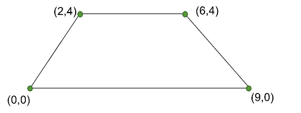
but this function returns a square (or isotropic if it is also valid) random field, what if one wants to generate a Random field input based on a certain FEM geometry (several coordinates) and different mesh sizes as similar to the attached figure, then what is the right replacement for the above?
I really appreciate your answer and others as well.