First of all, I am very grateful to uqlab for providing great convenience to my research.
Recently, I am using the PCE accelerated Bayesian inference module in uqlab to conduct research on my subject(Inversion of dam dynamic parameters), and I ran into some problems during this process.
Here is a description of my analysis:
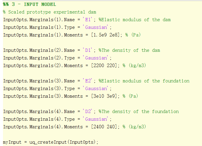
I have four inputs, as follows:
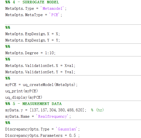
My model comes from a finite element software (ANSYS), with six outputs, which are the first six measured natural frequencies of the dam. It is surrogated with a PCE metamodel (Eloo ~ 6.26e-06 / 3.90e-06 / 5.57e-06 / 5.74e-06 / 0.0014 / 0.0165 for six outputs).
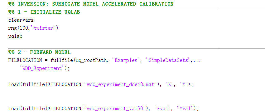
I use the calculation results from ANSYS and the input parameters from LHS sampling to construct the PCE, then use the measured data for inversion.
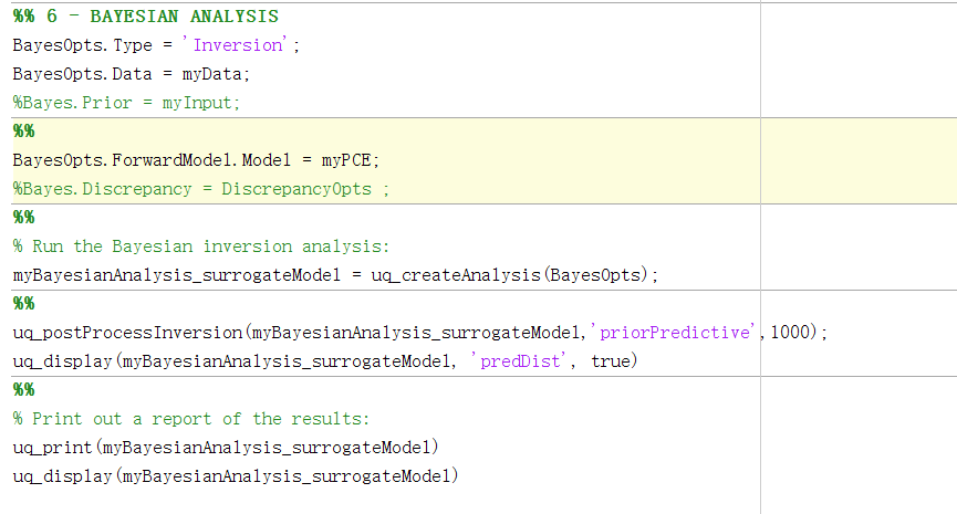
The complete code is as follows:
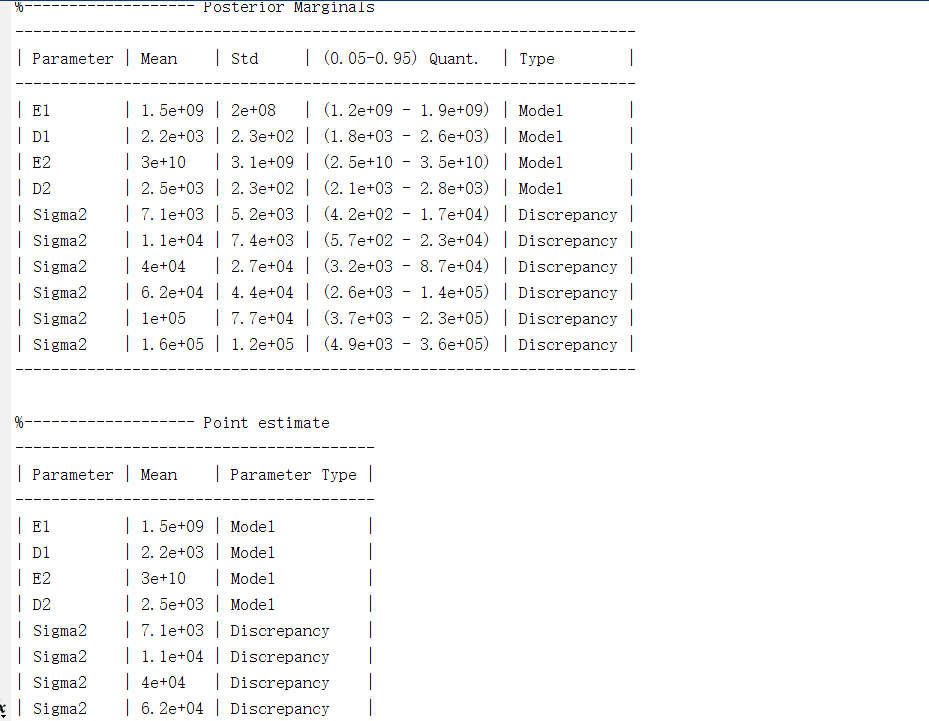
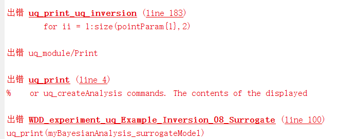
The calculation results in uqlab are as follows:
From the calculation results, we can see that the variance is very huge, But I don’t know what caused this result.
In addition, I would like to ask whether the posterior margins calculated by uqlab can be used to obtain specific posterior estimates,because what I have obtained is the specific posterior estimated value based on the program I wrote, as follows:
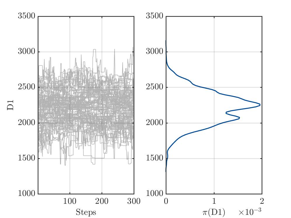
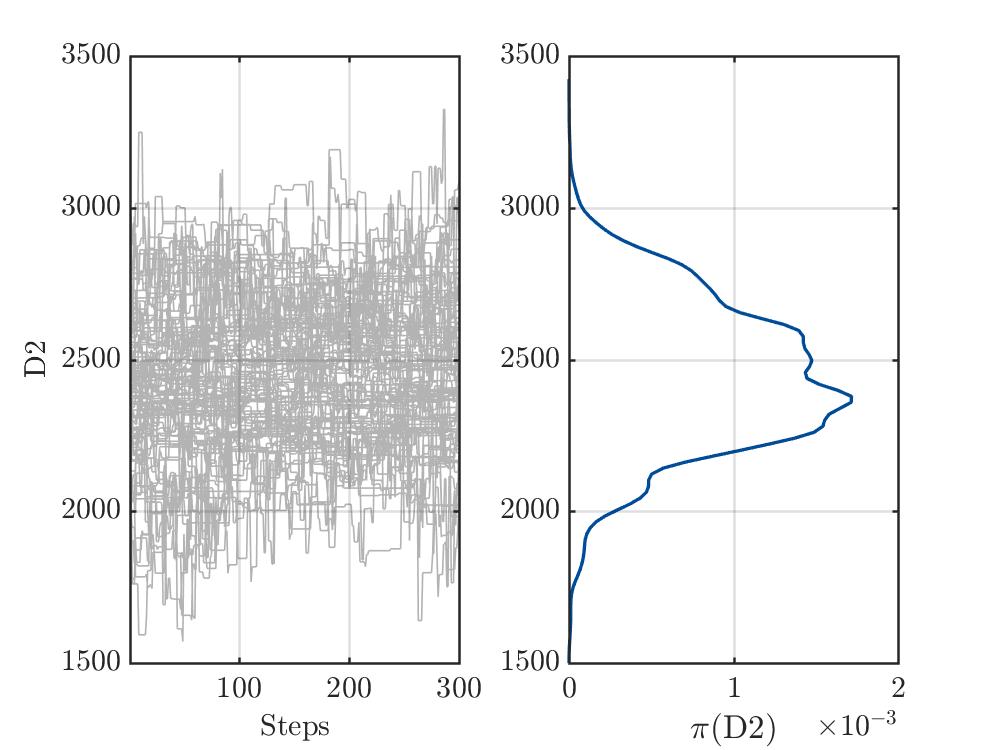
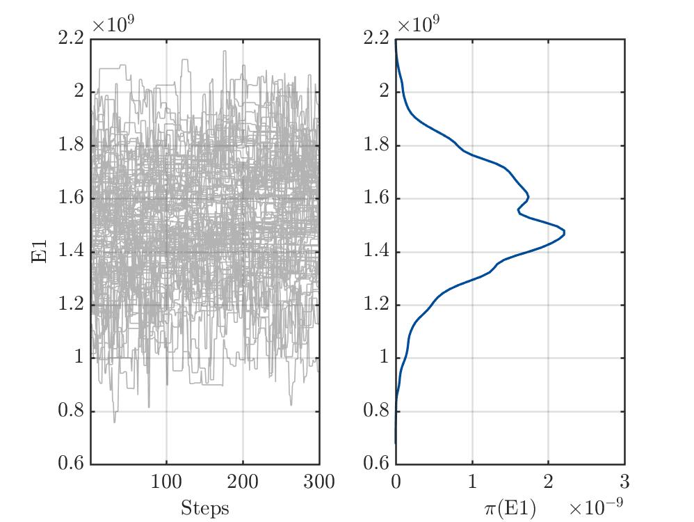
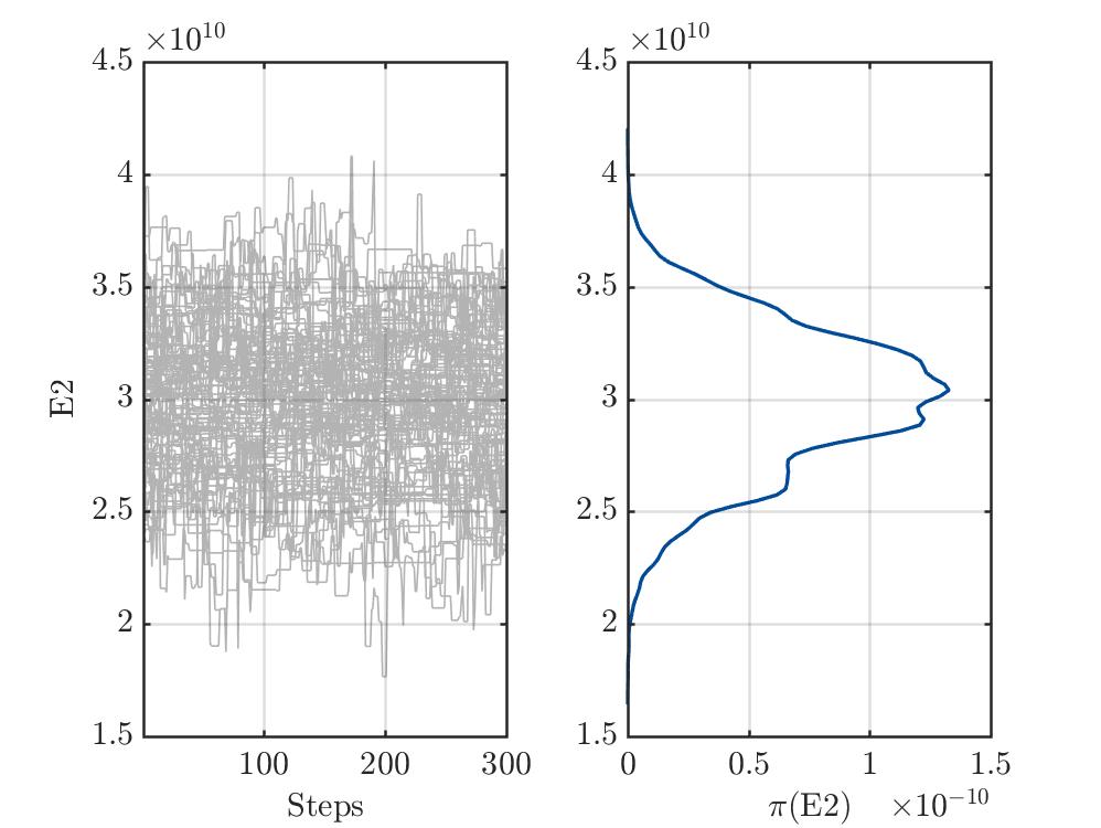
Your problem setup looks correct. However, from the information you provide it is difficult to say whether your MCMC chains have converged to the posterior distribution.
Could you also share trace Plots of the MCMC chains using the uq_display command?
P.S.: When sharing code, avoid using screenshots as they are not searchable/copyable. Either attach the files to the post or enclose the code in a pair of three apostrophes.
The values for mean and standard deviation for 'E1', 'D1', 'E2'and 'D2' provided in the definition of the prior measure are almost the same as the values in the chart computed from the posterior density.
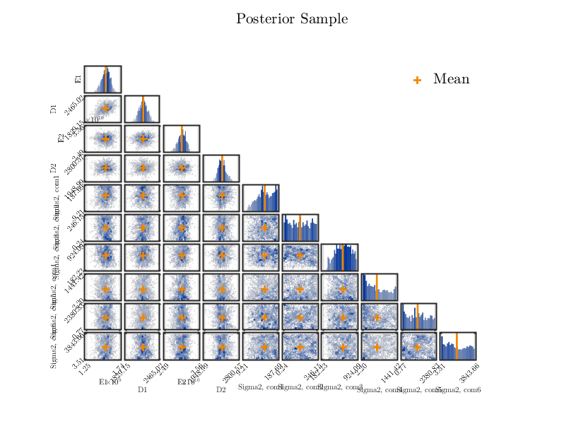
Since your setings for the discrepancy are not copied to BayesOpts.Discrepancy, UQLab follows it default setings, see Section 2.2.5 of the UQLab Bayesian Inversion Manual. In your situations this yields that UQLab assume that the error is an unknown additive Gaussian discrepancy term, and the prior distribution for \sigma^2 is uniform on [0,137^2] in the error for the first frequency, and for the 2nd to 6th inteveral we have [0,157^2], [0,304^2], [0,380^2], [0,488^2] ,[0,620^2]. Considering the mean and the standard deviation resulting from these distributions one can deduce that they are quite similar to the corresponding values for sigma2 in the charts in your results one realizes that the values are quite similar,
Combing point 1 and 2 it seems that the prior density and the posterior density are quite similar. So either the scheme has not converged yet as Paul-Remo Wagner has pointed as possibility (in view for your recent trace plots, I suggest to increase the number of steps ) or that the variation of the likelihood function is small, or that the likelihood shows large variations only in some region with quite small discrepancy values and the MCMC-scheme is not able to find this region since it is small compared to the domain considered in the computations.
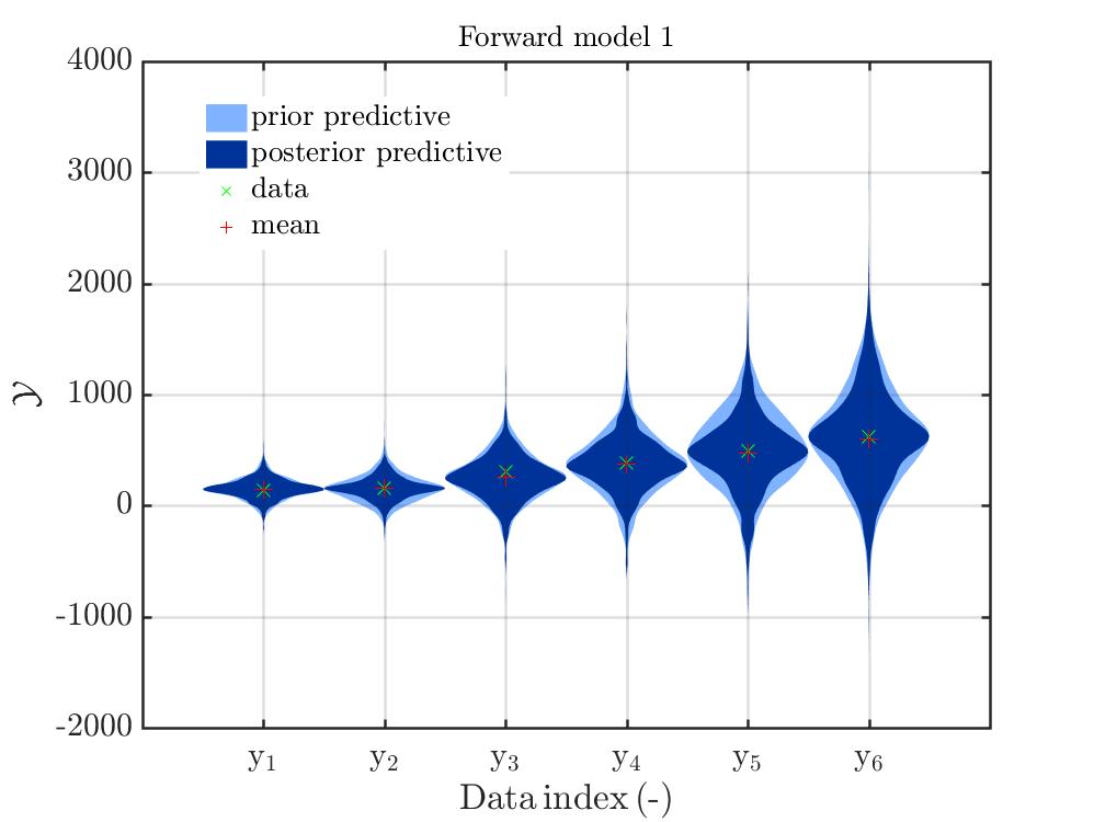
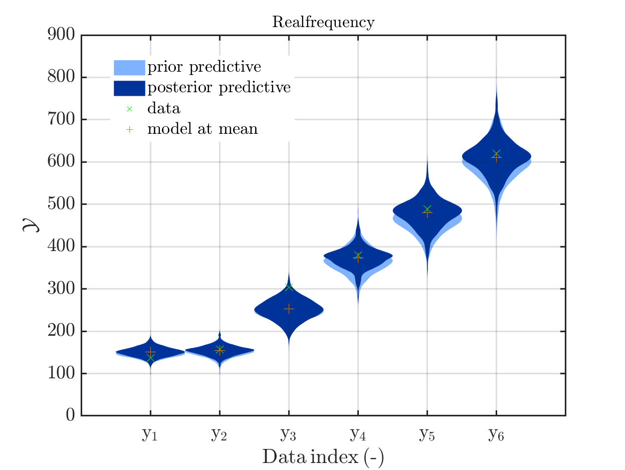
In view of the values for sigma2 discussed in point 2 it follows that noise added to the result of the model during the computation of the posterior density will quite large, leading to the large variation observed. (To be able to get plots to investigate the variations of the model output without noise, I suggest to update your UQLab version to 1.4.0 and to follow the instruction in my topic afterwards. )
It seems that the model output at the mean of the posterior density (which is marked by mean in your plots) is a quite good approximation of the measurement. And since the mean of the posterior density is almost identical to the mean of your prior density this should also hold for this mean.
Hence, I suggest to compare the Realfrequency vector with the output of the surrogate model (i.e. the output of uq_evalModel( myPCE,[1.5E9 2200 3e10 2400]); or uq_evalModel( myPCE,[1.5E9 ,2200, 3e10, 2400]);) and with the output of your finite element software at this point. And using this difference, one may get a better idea for the form of the discrepancy and the corresponding prior distribution, such that the likelihood function may show larger variations leading to posterior density being more different from the prior density.
I thinks that it is problem if the discrepancies sizes for all components are independent and
use therefore one discrepancy size for all components. But, I am not sure if this was really the best idea, since the size of different components differ such that maybe the size of the added noise should be proportional to the size of the measured value, but I am not sure. Maybe @paulremo has a some suggestion.
Hi,@olaf.klein
Thank you very much for your meticulous and thoughtful advice,and my gratitude is beyond words.
I will carefully consider your valuable suggestions for follow-up research.
When I updated uqlab, and combined with 2.2.5/2.2.6 of the UQLab Bayesian Inversion Manual, the following code was added:
I am sorry that my remark to section 2.2.5 of the manual generated confusion. I did not want to suggest to use this prior I just wanted to point out what UQLab does by default, at least according to the documentations.
Have you tried to run your old code without changes using UQLab V 1.4? Are there any problems?
If you really want to rebuild the internal UQLab default behavior you should follow the discussion in Section 2.3.4.2 of the Manual. I think that your code should look like the following to simulate this behavior:
This code should run and should allow to reproduce the default UQLab behavior.
But, I suggest to use other upper bound for the marginals. For example, assuming that you have a relative error of 10 % could be represented by multiplying the upper boundaries by 0.01.
3. If you would like to have one common discrepancy size for all components, you could try:
I added ‘DiscrepancyPriorOpts‘(from your reply) to my code ,
First, I used UQLab V 1.4 for calculations, and found that the error was the same as my previous reply.
When I returned to UQLab V 1.3, normal operation can be performed only Known residual variance is used, but the result has not changed from the previous.
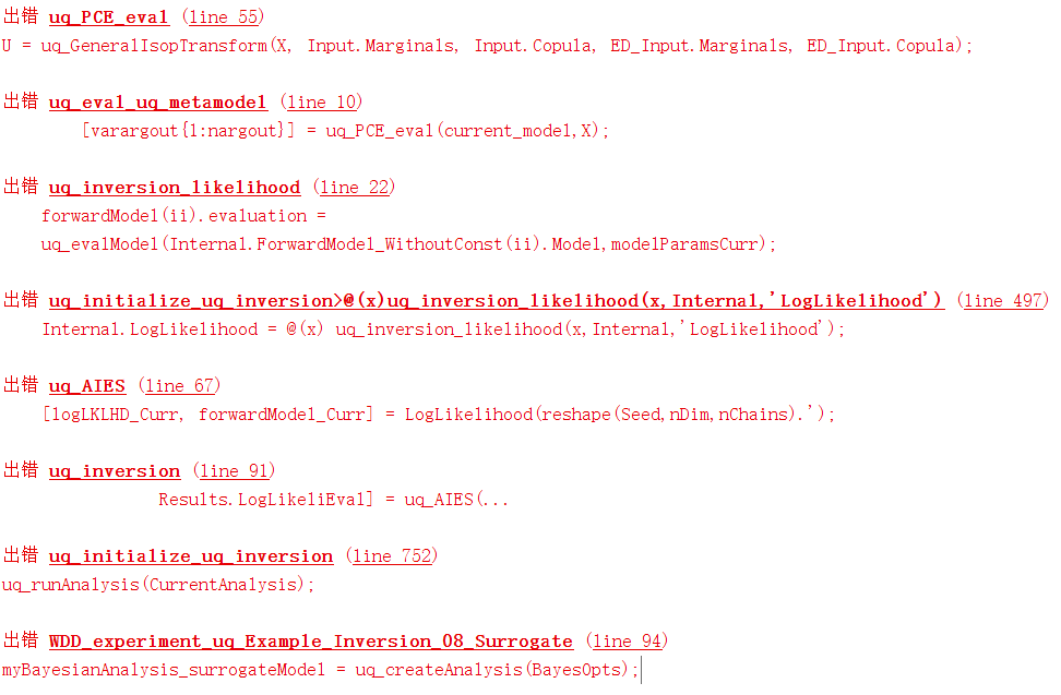
I have tested now both of your zip-Files and could run the version of WDD_experiment_uq_Example_Inversion_08_Surrogate_mod.m in the first zip-File after adapting the load command on with my UQLAB 1.3 and my UQLab 1.4 copy but starting the version of this file from the second zip file created the error mentioned by you for both UQLab versions.
Careful investigation of the difference between these files yields that you run in a side-effect of the UQLab-Feature to use the last created input model as prior distribution if no prior is provided in the input for uq_createAnalysis, see Sec. 2.2.5 of the manual. This works fine in the first version of your file but in the second version of the file the last created input model is the prior density for the discrepancy. To solve this problem, you should replace `
%Bayes.Prior = myInput;`
by
BayesOpts.Prior = myInput;
to explicitly define the prior for the parameters. And to use the settings for the discrepancy you have to add
BayesOpts.Discrepancy = DiscrepancyOpts
Adapting also settings for the discrepancy, see WDD_experiment_uq_Example_Inversion_08_Surrogate_third.m (5.6 KB)
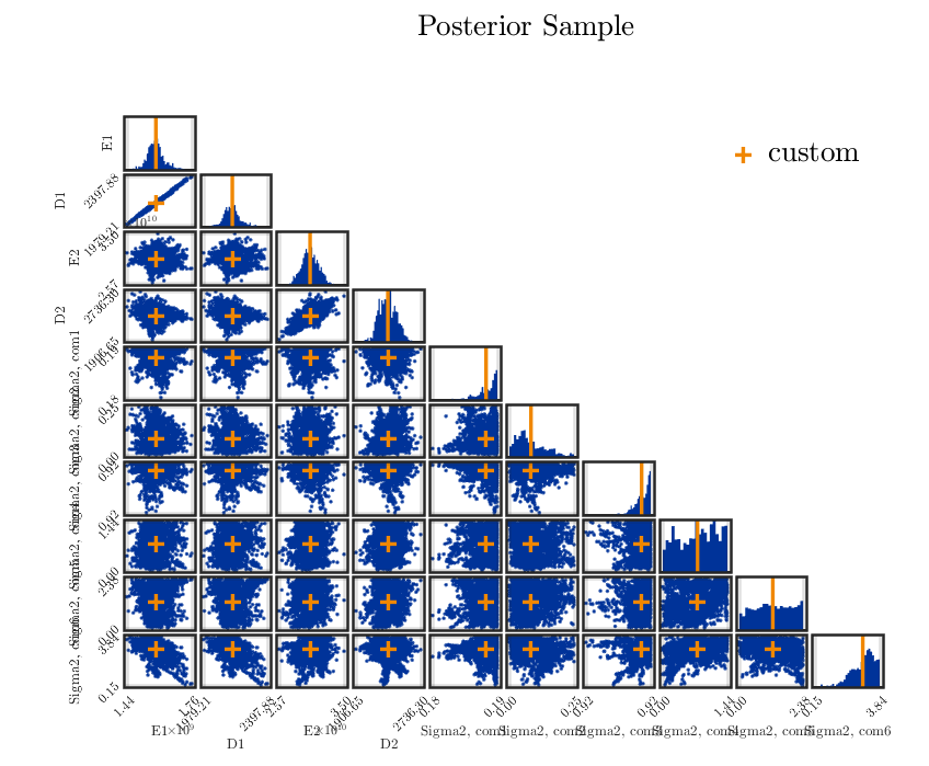
I could derive some results with a smaller variance since my settings are smaller then the
default UQLab settings (see above):
In view of the posterior sample plot, I think that one may be able to replace 0.01 by
a smaller factor for the discrepancy in the 2nd, 4th, 5th and 6th component, but this you should investigate.
Following your suggestion, I used many sets of smaller factor for the discrepance to test. It is found that although the variance and the confidence interval are slightly different, the point estimate is still only minor changes compared to the prior distribution, so this result may be difficult to be substituted into the FE model for model modification.
I believe there are many places worthy of my research, and I will carefully study the user manual of Bayesian inversion.
All in all, I am extremely grateful for your help.
it seems that you are in the somehow frustrating situation that the mean of your prior density is already a quite good approximation of the material data such that further inverse UQ computations do not allow to improve this data significantly. This may be the case if measurements for this dam/the material of the dam and of the foundation have already been used to create your original prior density.
My suggestions would be
Check that considering your situation with a prior being uniform on some appropriate set allows to generated a posterior density that is somehow similar to the prior density that you used above to show that this kind of identification works.
You may have to consider measurements for an other dam where the material data may be different and are not already known, e.g. an old dam such that the material in the center of the dam or of the foundation may have changed due to aging and one does not want to drill holes in the dam/the foundation to get samples of this material.
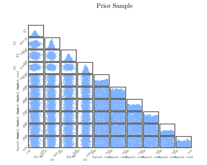
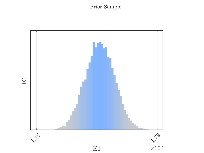
After running uq_Example_Inversion_08_Surrogate.m, the results of the prior distribution and posterior distribution are usually as follows:
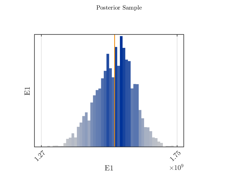
The information shown in this picture is amazing, but if I only want to display the comparison of a priori\posterior distribution of a certain parameter (as shown below), can uqlab achieve the results I want?
I checked UserManual_Bayesian carefully, it seems that there is no relevant introduction about it , but I think it is very interesting and meaningful to realize the tiny step.
I think that there are some UQLab featrues that may help you out of the box, but I am not sure if they
are sufficient for you.
One remark in advance.:
It holds in both for your files that your settings for Solver are not copied to BayesOpts.Solver at the end (see UQLab Manual 3.1.4) such that all your settings are ignored at the end and the default values are used. This can be seen for example in the trace plots above ending after 300 steps.
If you want, for example, compare the prior and posterior density for E1, you can use the commands
% Using the default value of  BayesOpts.Solver.MCMC.Steps being 300, the
% default value of  BayesOpst.Solver.MCMC.NChains being 100  for the default
% AIES-MCMC scheme and the default value of 0.5 for burnIn there are  151
% steps in  myBayesianAnalysis_surrogateModel.Results.PostProc.PostSample
% each with 100 values, i.e. there are 15100 samples values for the posterior
% densithy that are provided as input data to the plot function. To get plots
% that can be compared, we need a similar number  samples for the prior
% that are generated by the following call of uq_postProcessInversion
% Attention: In the following line there was an incorrect 5000 in the original version of this post
 uq_postProcessInversion(myBayesianAnalysis_surrogateModel,'prior',15100);
uq_display(myBayesianAnalysis_surrogateModel,'scatterplot',1)
leading to two figures similar to
and .
In the original UQLab 1.4.0 version of uq_display_uq_inversion.m the limits for the plots for the posterior density are determined from the limits for the plots for prior density, see my topic to this behavior. Hence, you can use these plots to compare prior and posterior densities.
In view of the plots above your may need more samples for both densities to get nice plots for both densities.
I would not be surprised if there are MATLAB methods to combine the two figures created by uq_display via calling uq_display_uq_inversion somehow after you managed to get the handles for them but this is beyond my MATLAB skill.
An other way to get one plot with prior and posterior density is (after following step 3) to copy the contents of myBayesianAnalysis_surrogateModel.Results.PostProc.PriorSample and of myBayesianAnalysis_surrogateModel.Results.PostProc.PostSample, following the instructions by Paul-Remo to rearrange the copy of ....PostSampe and use afterwards the MATLAB command histogram to generate a plot with histograms for both data sets.
 .
.