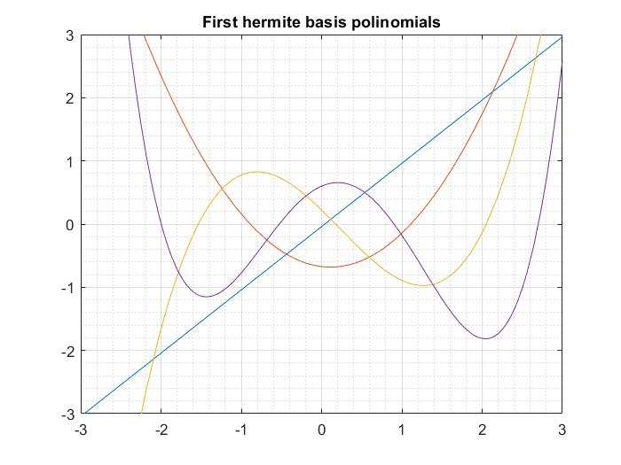
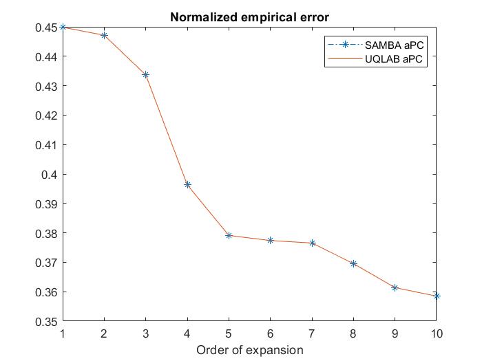
As promised I share here a performance test of aPC throught the method of moments available in the paper “SAMBA” against UQLAB aPC. With UQLAB aPC I mean to apply kernel estimation of the input marginals and Stieltjes procedure for the coefficients of the polynomials. Surprisingly, at least for one dimension, SAMBA and UQLAB have the same performance in terms of the so-called Normalized empirical error:
As can be seen in the attached code an picky input random variable is chosen and no less picky Y=M(X):
% Input X | Experimental design
ber= binornd(1,0.5,n,1); % Bernoulli rv
X=normrnd(0,3,n,1).*ber + (1-ber).*normrnd(5,1,n,1).^2+ ...
    5*sin( rand(n,1)*2*pi );

% Output Y | Experimental design
Y=exp(-abs(X))+sin(-X)+log(abs(X)+1);
Complete code ( I can’t attach it since it says “new users can not upload attachments”):
%%%%% aPC expansion: SAMBA vs UQLAB-KS %%%%%
%% Main parameters
clearvars
rng(100,'twister');
n=2e3; % Data size
nVal=1e3; % Validation data size
n_order=10; % Arbitrary Polynomial expansion order

%% Experimental design
% Input X | Experimental design
ber= binornd(1,0.5,n,1); % Bernoulli rv
X=normrnd(0,3,n,1).*ber + (1-ber).*normrnd(5,1,n,1).^2+ ...
    5*sin( rand(n,1)*2*pi );

% Output Y | Experimental design
Y=exp(-abs(X))+sin(-X)+log(abs(X)+1);

% Validation sets
XVal=linspace(min(X), max(X), nVal)';
YVal=exp(-abs(XVal))+sin(-XVal)+log(abs(XVal)+1);
%% aPC: UQLAB vs SAMBA Moments PC (non sparse version)
syms x
Ypc=zeros(1,n); YpcVal=zeros(1,nVal);
samba_er=zeros(1,n_order); uq_erVal=zeros(1,n_order);
uq_er=zeros(1,n_order);
for p=1:n_order
    %% Samba
    Pn=sPC_poly(X,p);
    Pn_fun=matlabFunction(Pn);
    A=zeros(n,p+1);
    for i=1:n
        A(i,:)=Pn_fun(X(i));
    end
    % Regresion
    alpha=(A'*A)\(A'*Y);

    % Y_hat through SAMBA
    for i=1:n
        Ypc(i)=sum(alpha'.*Pn_fun(X(i)));
    end
    samba_er(p)=sum((Y-Ypc').^2)/sum( (Y-mean(Y)).^2 );

    % Y_hat through SAMBA
    for i=1:nVal
        YpcVal(i)=sum(alpha'.*Pn_fun(XVal(i)));
    end
    samba_erVal(p)=sum((YVal-YpcVal').^2)/sum( (YVal-mean(YVal)).^2 );
    %% UQLAB aPC (Kernel  estimation of marginals)
    InputOpts.Marginals(1).Type = 'KS';
    InputOpts.Marginals(1).Parameters = X;
    % Create an INPUT object based on the specified marginals:
    myInput = uq_createInput(InputOpts);

    MetaOpts.Type = 'Metamodel';
    MetaOpts.MetaType = 'PCE';
    MetaOpts.Method = 'OLS';

    MetaOpts.ExpDesign.X=X;
    MetaOpts.ExpDesign.Y=Y;

    MetaOpts.ValidationSet.X = XVal;
    MetaOpts.ValidationSet.Y = YVal;

    MetaOpts.Degree = p;
    myPCE = uq_createModel(MetaOpts);
    uq_er(p)=myPCE.Error.normEmpErr;
    uq_erVal(p)=myPCE.Error.Val;
end

%% Error representation
subplot(2,1,1)
plot(1:n_order,samba_er,'-.*',1:n_order,uq_er)
xlabel('Order of expansion')
title('Normalized empirical error TRAIN')
legend('SAMBA aPC', 'UQLAB aPC')

subplot(2,1,2)
plot(1:n_order,samba_erVal,'-.*',1:n_order,uq_erVal)
xlabel('Order of expansion')
title('Normalized empirical error VALIDATION')
legend('SAMBA aPC', 'UQLAB aPC')
    indent preformatted text by 4 spaces
Auxiliar function needed for SAMBA methodology:
function [p]=sPC_poly(X,n) % Samba
%% We computes the first 2n moments
M=zeros(n+1,n+1); % Hankel Matrix of moments
m=zeros(1,2*n+1)'; % Moments vector. m(k)= moment k+1

n_x=length(X);
m(1)=1;
for i=1: (n-1)
    m(i+1)=sum(X.^i)/n_x;
end

for i=(n: 2*n)
    m(i+1)=sum(X.^i)/n_x;
    M(:,i-n+1)=m(i-n+1 : i+1);
end

if det(M)<=0
    warning(['Determinant of Hankel Matrix:' num2str(det(M))])
end

%% We find the Cholesky descomposition of the Hankel matrix of moments
% and find the coeficientes with the three term recurrence relationship:

R=chol(M);
a=zeros(n,1);
b=zeros(n,1);
a(1)=R(1,2)/R(1,1)-0/1;
b(1)=R(2,2)/R(1,1);
for i=2:n % Order of R matrix: n+1,n+1
    a(i)=R(i,i+1)/R(i,i)-R(i-1,i)/R(i-1,i-1);
    b(i)=R(i+1,i+1)/R(i,i);
end
% J=diag(a)+diag(b(1:(n-1)),-1)+diag(b(1:(n-1)),1);

syms x
p(1)=sym(1); % Orden 0. Como siempre son ortogonales pol=1 (dFx);
p(2)=(x-a(1))/b(1);

if n>1 % p(i)= pol de orden i-1
   %  p(3)=(x-a(2))/b(2)*p(2) - b(1)/b(2)*1;  % a(j)=a_j. b(j)=b_j
    for j=2:n
        p(j+1)=(x-a(j))/b(j)*p(j) - b(j-1)/b(j)*p(j-1); % p(j)=phi_{j-1}
    end
end