Unexpected Behavior in Bayesian Inversion using GPR Surrogate

David · February 27, 2022, 4:01pm

Dear Community

My name is David and I’m trying to use the Bayesian Inversion module of UQLab to calibrate some model parameters for my physics-based system. I’m new in this field and have now some problems, where I need some guidance from your side to interprete and improve the results.

Background:
My goal is to derive point estimates (e.g. MAP) together with uncertainty bounds (e.g. percentile credible intervals) for some model parameters (N_model=3) used in a radiation transport Monte Carlo code. The ouptut of the radiation transport code is a pulse-height spectrum with 1024 channels. I’m extracting only a small part of this spectrum for the Bayesian Inversion analysis (73 channels), because the observed model parameters have only a significant impact in this small region (N_output=73).

Probabilistic Model:
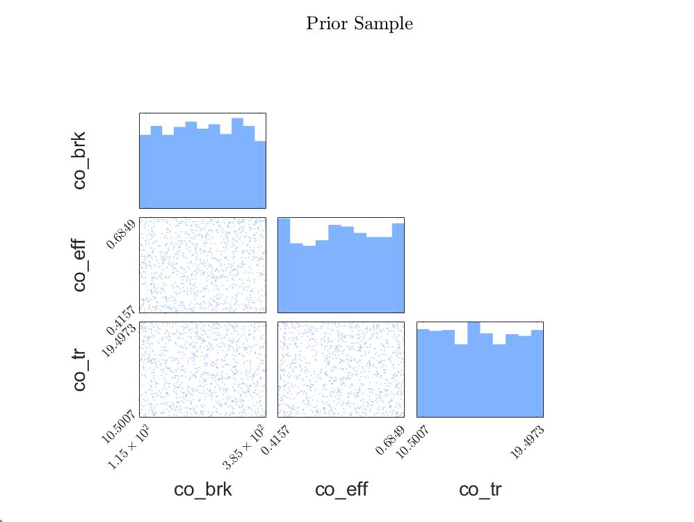
The probabilistic model adopted for the three parameters is physics-motivated, i.e. literature values were gathered and a conservative upper and lower limit for each parameter was defined. The marginal distribution for the parameters is assumed to be uniform due to the lack of more detailed information (maximum entropy principle).


%%%%%%%%%%%%%%%%%%%%%%%%%%%%%%%%%%%%%%%%%%%%%%%%%%%%%%%%%%%%%%%%%%%%%%%%%%
%%-------------------- Define Probabilistic Input Model ----------------%%
%%%%%%%%%%%%%%%%%%%%%%%%%%%%%%%%%%%%%%%%%%%%%%%%%%%%%%%%%%%%%%%%%%%%%%%%%%

%% 1) Command Line Output
disp(['Define Probabilistic Input Model , ' char(datetime)]);

%% 2) Define Probabilistic Model

% i) Birks coefficient
Input.Marginals(1).Type = 'Uniform';
Input.Marginals(1).Parameters = [100 400];                                  % [MeV/cm]
Input.Marginals(1).Name='co_brk';

% ii) Onsager coefficient
Input.Marginals(2).Type = 'Constant';
Input.Marginals(2).Parameters = 36.4;                                       % [MeV/cm]
Input.Marginals(2).Name='co_ons';

% iii) Free electron/hole formation efficiency coefficient
Input.Marginals(3).Type = 'Uniform';
Input.Marginals(3).Parameters = [0.35 0.65];                                 % [-]
Input.Marginals(3).Name='co_eff';

% iv) Debye-related trapping coefficient
Input.Marginals(4).Type = 'Uniform';
Input.Marginals(4).Parameters = [10 30];                                    % [MeV/cm]
Input.Marginals(4).Name='co_tr';
Input.Name='ProbModel_v1';
Input.Copula.Type = 'Independent';

%% 3) Create Probabilistic Model
ProbModel = uq_createInput(Input);

Forward Model:
Based on the probabilistic model, I have performed 100 simulation with a predefined experimental design (LHC sampling). Due to the fact that 1 datapoint takes about 1h on a computer cluster, I have trained a Gaussian Process Regression surrogate using the Kriging module of UQLab. The mean relative validation error (using 10 validation data points) for all 73 channels is <3%, which was judged to be sufficient for a preliminary test.

It is worth noting that I have performed principle component analysis (PCA) to reduce the number of output dimensions for the surrogate model from 73 to 4 using a threshold of 99% for the relative explained variance. The mean validation error mentioned before is of course evaluated on the (back-transformed) original data space. The surrogate model consists therefore of 4 GPR models and the PCA transformation matrix (T).

Experimental data:
The radiation transport code mentioned before is used to simulate a radiation measurement, which I have performed. The experimental data consists of a 1 x 73 data array, i.e. 73 channels (N_output=73) and 1 independent measurement (N=1).

Bayesian Inversion:
The Bayesian Inversion is performed using the Bayesian Inversion module of UQLab. I’ve adopted the AIES MCMC solver with 10^2 chains and 5*10^4 steps. For the prior model, the same probabilistic model as for the derivation of the surrogate model was used. For the forward model, the trained and validated GPR model is used. For the postprocessing, a burn-in fraction of 0.5 was used. For the discrepancy model, the default zero-mean Gaussian model with unknown sigma2 parameters was used. The script to perform the Bayesian Inversion is attached at the end of this post.

Problems:

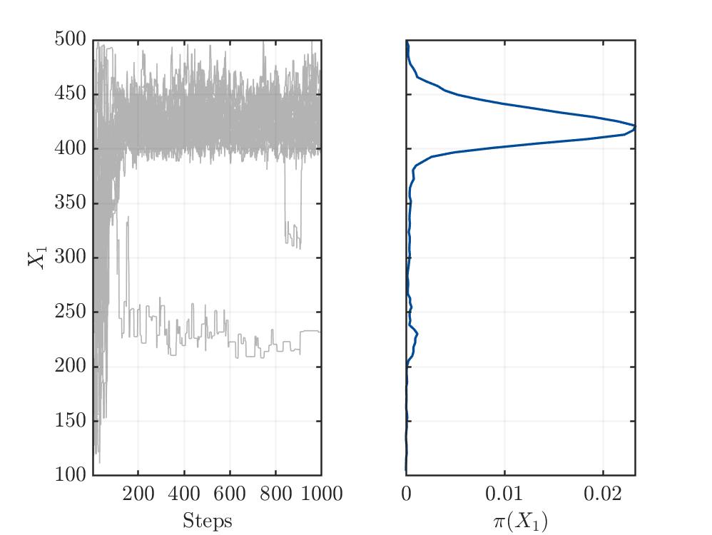
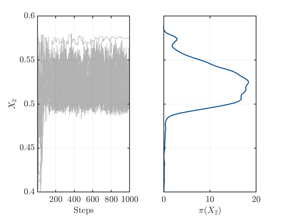
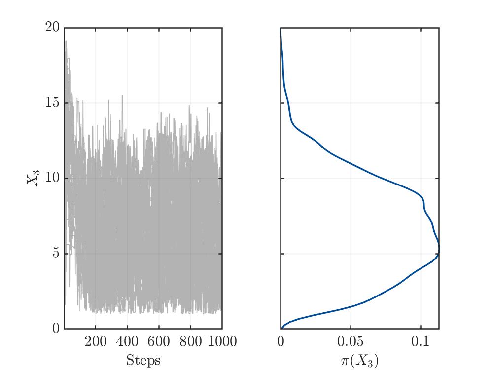
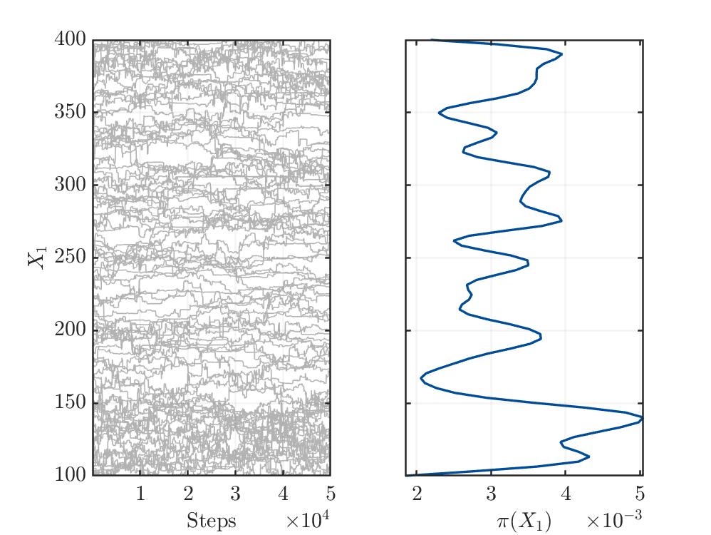
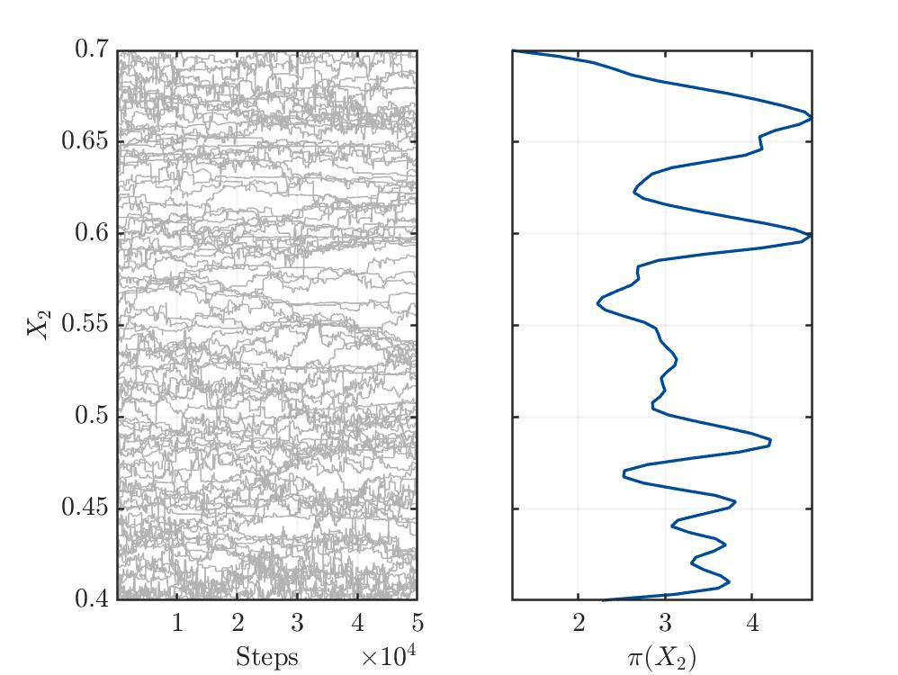
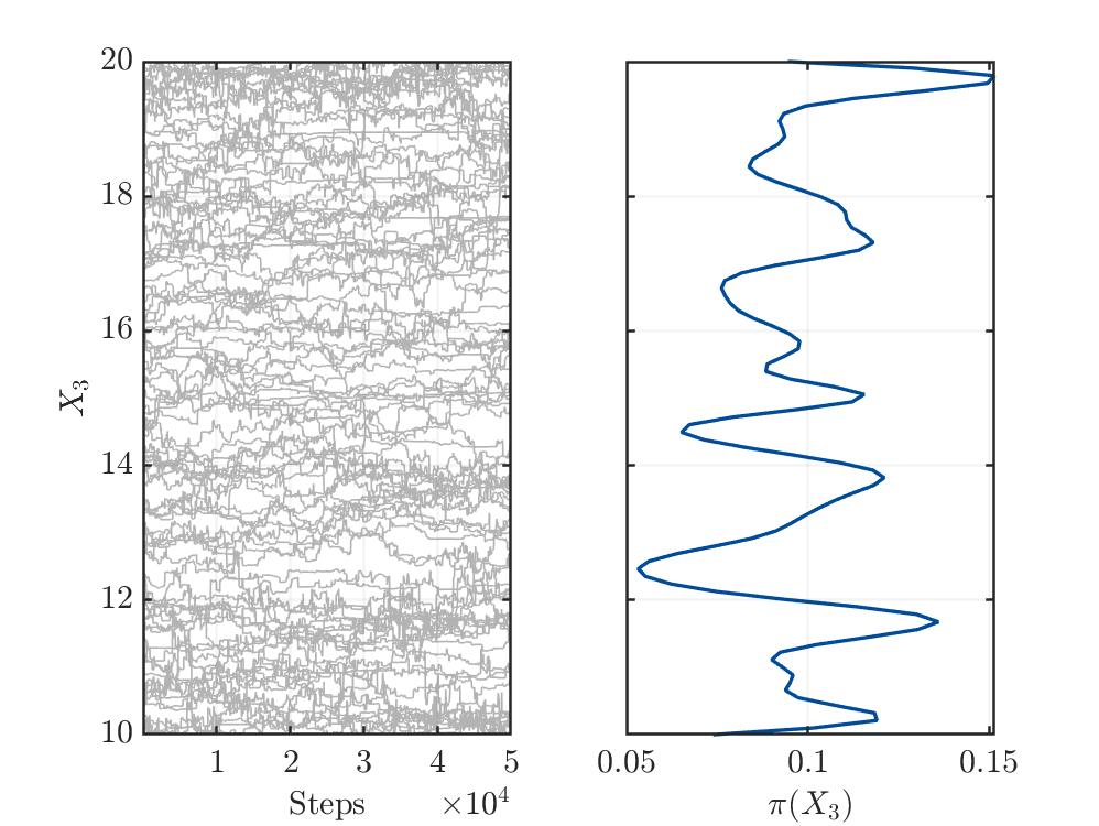
I’m not sure, but from my limited understanding, the trace plots (see below) for the three variables show no convergence. This might indicate a bad setup of the MCMC solver or something else, which I’m not aware.
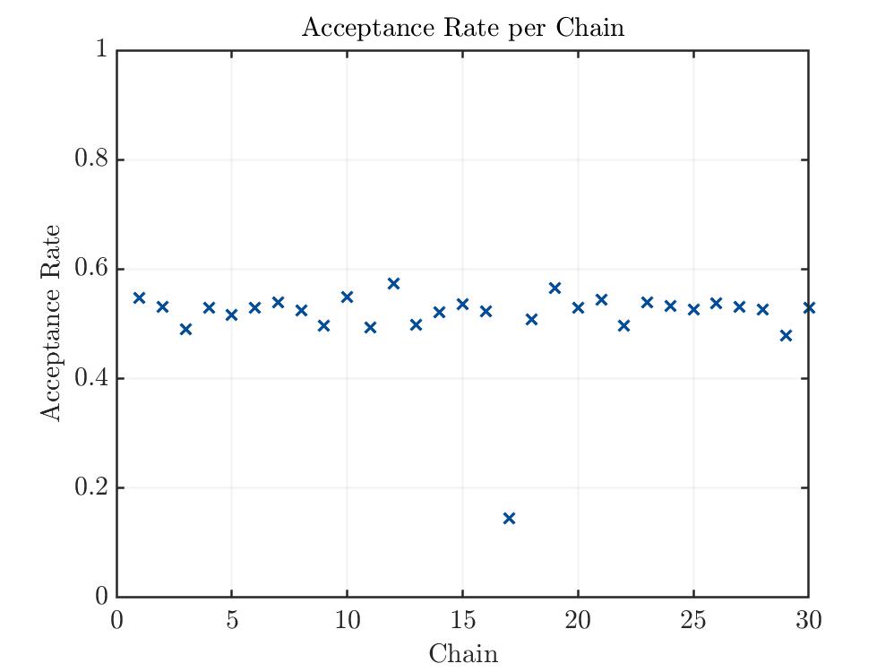
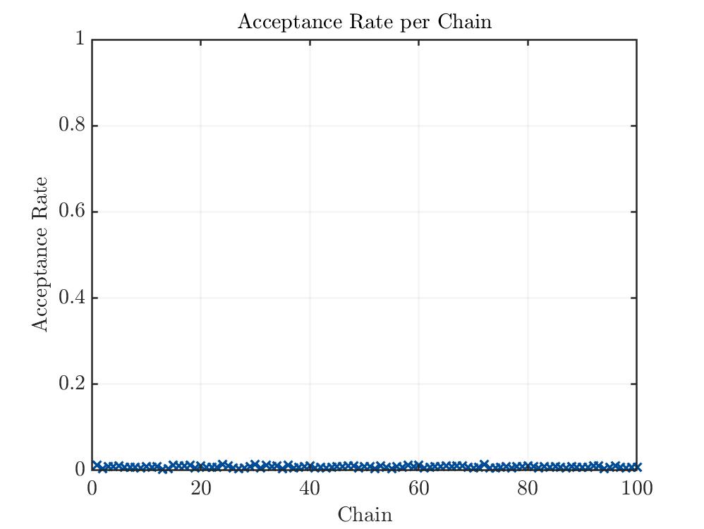
The acceptance rate is in my opinion way to low.
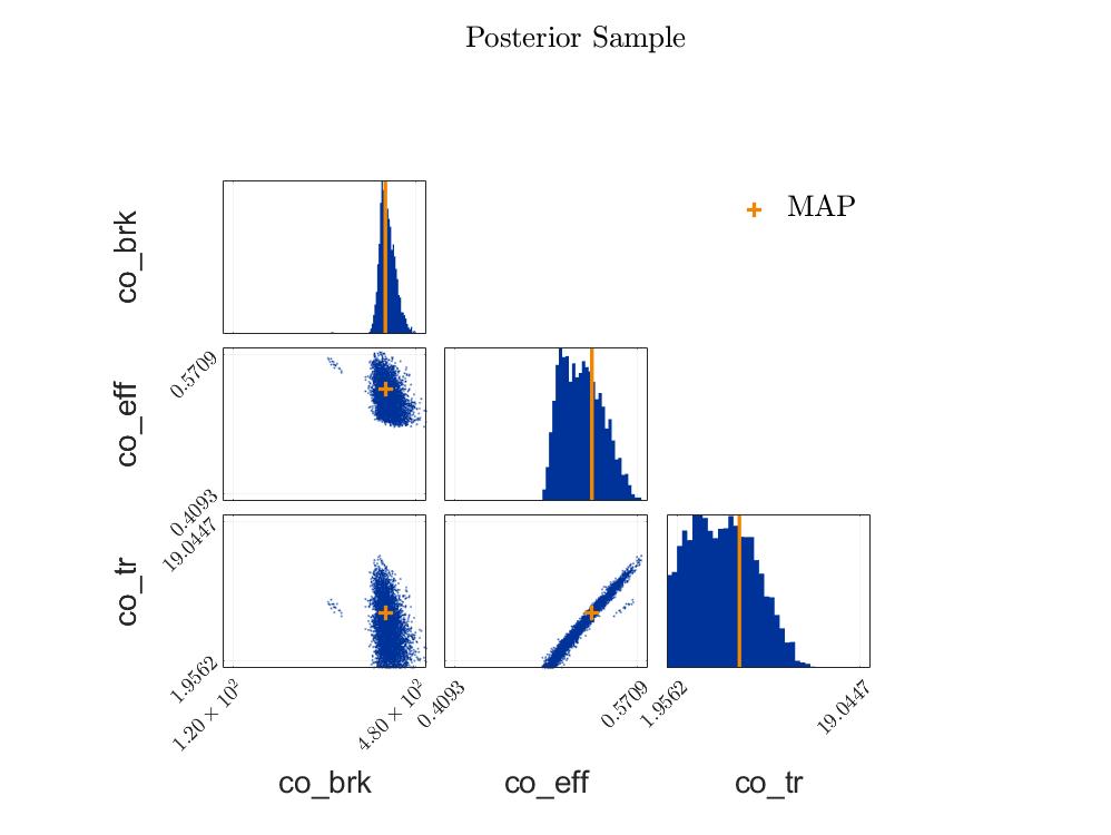
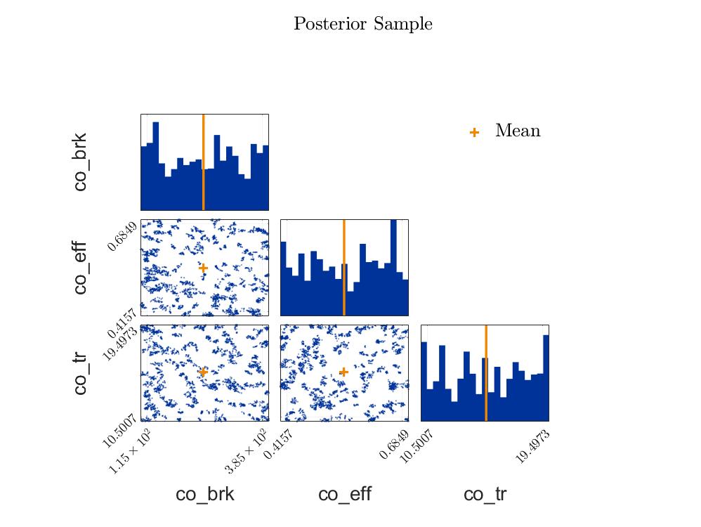
The posterior samples show a strange clustering.

This three points indicate, at least in my understanding, a problem with the setup of the MCMC solver.

Further analysis:
I tried the following things to investigate and improve the perfomance of the code:

Use different discrepancy models, i.e. (a) only 1 sigma2 variable and (b) a different prior distribution for the sigma2 variables, i.e. an exponential distribution with a mean = mean(Y).
Adapt the AIES model parameter a (I changed it from 2 to 50).
Use a different MCMC solver, i.e. I used the default HMC solver.
I used the surrogate with no PCA reduction, i.e. I kept the 73 output dimensions
Use only 2 input dimensions, i.e. fix the third input parameter.

Unfortunately, none of these changes improved the behavior of the algorithm.

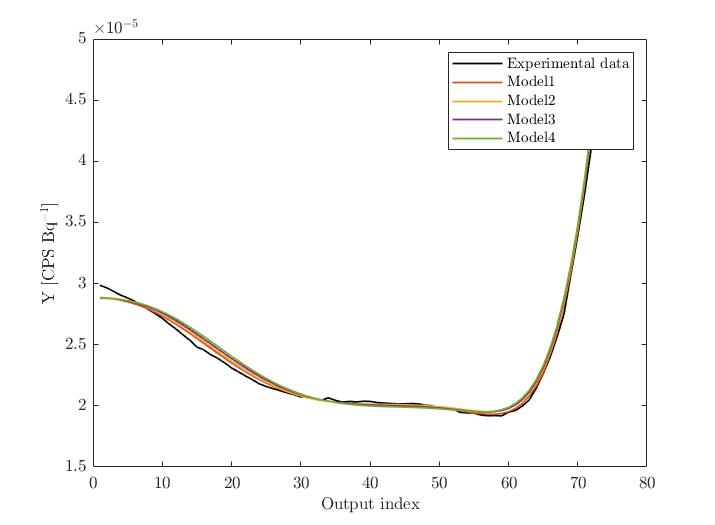
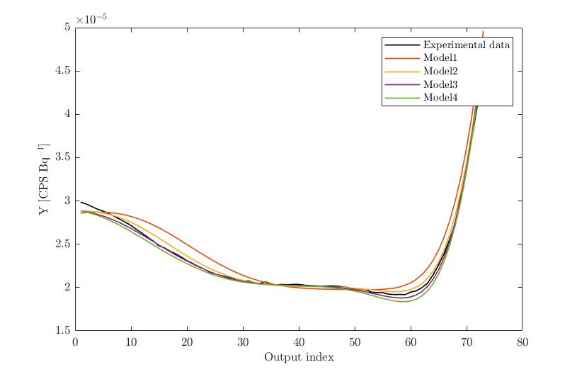
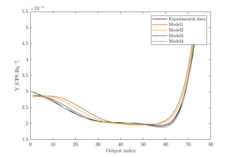
To get more insights in my problem, I’ve also plotted the experimental data together with some selected model evaluations covering the entire parameter space (I have altered one parameter at the time). The results show that the model evaluations are indeed covering the experimental data, i.e. I would expect that the BAyesian Inversion finds some particular MAP, but for sure not a simple uniform posterior distribution for all model parameters.

Questions:

Do you agree with me that the results indicate nonconvergence of the MCMC solver?
If the answer is yes to the first question: what is the reason for this “bad” behavior? Is there a bug in my code? Do I have to generate more steps? In my opinion, there is no trend at all in the trace plots, which would indicate a convergence anytime soon.
What can I do to improve the convergence behavior of the MCMC solver?
Could it be that my problem here is somewhat ill-posed or simply particularly difficult to solve? In my opinion, the plots “experimental data vs. model evaluations” (discussed in the previous section) indicate that there should be some MAP, i.e. a more or less unimodel posterior distribution. In addition, the examples for Bayesian Inversion highlighted at the UQLab homepage indicate that also with only 1 independent measurement, powerfull Bayesian Inference can be performed (e.g. the hydro example). So I don’t expect that the fact that I have only 1 independent data, is the reason for the bad convergence.
Could there be some numerical problems with the units/order of magnitude of the ouptut (~10^-5)? Should I perform some sort of standardization (e.g. (Y-mean(Y))/std(Y)) before performing the Bayesian inversion (i did of course perform standardization for the GPR training)?
Is my general workflow correct to perform the Bayesian Inversion in my specific case or do you suggest some other or altered steps, e.g. use the output dimension/channel index as an additional input, which would result in a single-output problem?
Should I try different prior distributions? As already said, I’m new in this field and have no experience, which prior distribution should be used for my specific problem.

Additional Notes:

For your convenience, I’m attaching all the scripts, data and images at the end of this post.
I’m using the newest version of UQLab, i.e. v2.0.
The Monte Carlo code simulations were performed on a computer cluster. The Bayesian Inversion was performed on my local computer.
Unfortunately, I can’t attach files directly to this post, because I’m a new user. Therefore, I used the Polybox repository.
One of the model parameters (Onsager coefficient) was fixed due to some references in the literature. This should not alter the performance of the Bayesian Inversion.
The ouptut unit (e.g. shown in the last three plots) is CPS Bq^-1, i.e. counts per second per source activity.

Thank you so much for your support
Cheers!
David

Attachment:

The scripts, data and model can be downloaded under the following repository:

The following script was used to perform the Bayesian Inversion:

%%%%%%%%%%%%%%%%%%%%%%%%%%%%%%%%%%%%%%%%%%%%%%%%%%%%%%%%%%%%%%%%%%%%%%%%%%
%%%%%%%%%%%%%%%%%%%%%%%%%%%%%%%%%%%%%%%%%%%%%%%%%%%%%%%%%%%%%%%%%%%%%%%%%%
% ======================== Bayesian Inversion ========================== %
%%%%%%%%%%%%%%%%%%%%%%%%%%%%%%%%%%%%%%%%%%%%%%%%%%%%%%%%%%%%%%%%%%%%%%%%%%
%%%%%%%%%%%%%%%%%%%%%%%%%%%%%%%%%%%%%%%%%%%%%%%%%%%%%%%%%%%%%%%%%%%%%%%%%%
%                                                                        %
%  27.02.2022                                                            %
%                                                                        %
%  Paul Scherrer Institut                                                %
%  David Breitenmoser                                                    %
%  OFLD/U06                                                              %
%  Forschungsstrasse 111                                                 %
%  5232 Villigen PSI                                                     %
%  Switzerland                                                           %
%                                                                        %
%  Phone: +41 56 310 44 61                                               %
%  E-Mail: david.breitenmoser@psi.ch                                     %
%                                                                        %
%                                                                        %
%                                                                        %
%  Description:                                                          %
%    Perform Bayesian Inversion                                          %
%                                                                        %
%                                                                        %
% Copyright (c) 2022, David Breitenmoser                                 %
% All rights reserved.                                                   %
%                                                                        %
% Redistribution and use in source and binary forms, with or without     %
% modification, are permitted provided that the following conditions are %
% met:                                                                   %
%                                                                        %
%     * Redistributions of source code must retain the above copyright   %
%       notice, this list of conditions and the following disclaimer.    %
%     * Redistributions in binary form must reproduce the above copyright%
%       notice, this list of conditions and the following disclaimer in  %
%       the documentation and/or other materials provided with the       %
%       distribution                                                     %
%                                                                        %
% THIS SOFTWARE IS PROVIDED BY THE COPYRIGHT HOLDERS AND CONTRIBUTORS "AS%
% IS" AND ANY EXPRESS OR IMPLIED WARRANTIES, INCLUDING, BUT NOT LIMITED  %
% TO, THE IMPLIED WARRANTIES OF MERCHANTABILITY AND FITNESS FOR A        %
% PARTICULAR PURPOSE ARE DISCLAIMED. IN NO EVENT SHALL THE COPYRIGHT     %
% OWNER OR CONTRIBUTORS BE LIABLE FOR ANY DIRECT, INDIRECT, INCIDENTAL,  %
% SPECIAL, EXEMPLARY, OR CONSEQUENTIAL DAMAGES (INCLUDING, BUT NOT       %
% LIMITED TO, PROCUREMENT OF SUBSTITUTE GOODS OR SERVICES; LOSS OF USE,  %
% DATA, OR PROFITS; OR BUSINESS INTERRUPTION) HOWEVER CAUSED AND ON ANY  %
% THEORY OF LIABILITY, WHETHER IN CONTRACT, STRICT LIABILITY, OR TORT    %
% (INCLUDING NEGLIGENCE OR OTHERWISE) ARISING IN ANY WAY OUT OF THE USE  %
% OF THIS SOFTWARE, EVEN IF ADVISED OF THE POSSIBILITY OF SUCH DAMAGE.   %
%                                                                        %
%%%%%%%%%%%%%%%%%%%%%%%%%%%%%%%%%%%%%%%%%%%%%%%%%%%%%%%%%%%%%%%%%%%%%%%%%%
%%%%%%%%%%%%%%%%%%%%%%%%%%%%%%%%%%%%%%%%%%%%%%%%%%%%%%%%%%%%%%%%%%%%%%%%%%


%%%%%%%%%%%%%%%%%%%%%%%%%%%%%%%%%%%%%%%%%%%%%%%%%%%%%%%%%%%%%%%%%%%%%%%%%%
%%----------------------------- Preparation ----------------------------%%
%%%%%%%%%%%%%%%%%%%%%%%%%%%%%%%%%%%%%%%%%%%%%%%%%%%%%%%%%%%%%%%%%%%%%%%%%%

%% --- tabula rasa ---
close all
clear variables
fclose('all');
clc

%% --- Change Default Values ---
set(groot,'defaulttextinterpreter','latex')
set(groot, 'defaultAxesTickLabelInterpreter','latex');
set(groot, 'defaultLegendInterpreter','latex');

set(0,'DefaultTextFontname', 'Latin Modern Roman')
set(0,'DefaultAxesFontName', 'Latin Modern Roman')
set(0,'DefaultLegendFontName','Latin Modern Roman');

set(0, 'DefaultLineLineWidth', 1);

%% --- Set random number generator for reproducable results ---
rng(100,'twister')

%% --- Initilaize UQlab ---
uqlab

%%%%%%%%%%%%%%%%%%%%%%%%%%%%%%%%%%%%%%%%%%%%%%%%%%%%%%%%%%%%%%%%%%%%%%%%%%
%%---------------------------- Input Deck ------------------------------%%
%%%%%%%%%%%%%%%%%%%%%%%%%%%%%%%%%%%%%%%%%%%%%%%%%%%%%%%%%%%%%%%%%%%%%%%%%%


%% 1) Input Folder
main_path=['J:\Datenanalyse\Intrinsic Resolution\Det4_October_2021\Bayesian_Approach'];
ProbMdl_path=[main_path '\ProbModel\ProbModel_v1.mat'];
ExpData_path=[main_path '\FLUKA\FLUKA_ExpDesign_v1_v4\Postprocessing\exp\v2\SPEC_response.mat'];
MetaModel_path=[main_path '\Emulator\FLUKA_ExpDesign_v1_v4\GPR\v2\GPR_model.mat'];

%% 2) Output Folder
output_path=[main_path '\Bayesian Inversion\FLUKA_ExpDesign_v1_v4\v1'];
CHECKfolder_v1(output_path)

%%%%%%%%%%%%%%%%%%%%%%%%%%%%%%%%%%%%%%%%%%%%%%%%%%%%%%%%%%%%%%%%%%%%%%%%%%
%%-------------------------------- Load Data ---------------------------%%
%%%%%%%%%%%%%%%%%%%%%%%%%%%%%%%%%%%%%%%%%%%%%%%%%%%%%%%%%%%%%%%%%%%%%%%%%%

%% 1) Load Probabilistic Input Model
disp(['Load Probabilistic Input Model , ' char(datetime)]);
load([ProbMdl_path])
N_var=length(ProbModel.nonConst);

%% 2) Load Experimental Data
disp(['Load Experimental Data , ' char(datetime)]);
load([ExpData_path],'Y')
N_det=size(Y.mean_exp.value,1);

%% 3) Load Metamodel
disp(['Load Metamodel , ' char(datetime)]);
load([MetaModel_path],'myGPR')


%%%%%%%%%%%%%%%%%%%%%%%%%%%%%%%%%%%%%%%%%%%%%%%%%%%%%%%%%%%%%%%%%%%%%%%%%%
%%---------------------- Perform Bayesian Inversion --------------------%%
%%%%%%%%%%%%%%%%%%%%%%%%%%%%%%%%%%%%%%%%%%%%%%%%%%%%%%%%%%%%%%%%%%%%%%%%%%

%% 1) Setup Bayesian Inversion Module
BayesOpts.Type = 'Inversion';
BayesOpts.Name=['BayesianInversion_det' num2str(round(1-1))];

%% 2) Experimental Data
BayesOpts.Data.y = Y.mean_exp.value{1,1}';
myData=BayesOpts.Data.y;
N_y=length(Y.mean_exp.value{1,1});

%% 3) Forward Model
modelopts.mFile='uq_PCA_evalModel';
modelopts.Parameters=myGPR{1,1};
myMeta=myGPR{1,1};
uq_myMdl=uq_createModel(modelopts);
BayesOpts.ForwardModel.Model = uq_myMdl;


%% 4) Prior Model
BayesOpts.Prior = ProbModel;

%% 6) Solver
BayesOpts.Solver.Type = 'MCMC';
BayesOpts.Solver.MCMC.Sampler = 'AIES';
BayesOpts.Solver.MCMC.NChains = 10^2;                                        % Number of parallel chains
BayesOpts.Solver.MCMC.Steps = 5*10^4;                                        % Number of iterations per chain
BayesOpts.Solver.MCMC.a=2;

BayesOpts.Solver.MCMC.Visualize.Parameters = [1:N_var];
BayesOpts.Solver.MCMC.Visualize.Interval = round(0.1*BayesOpts.Solver.MCMC.Steps);

%% 7) Execute Inversion
myBayesianAnalysis = uq_createAnalysis(BayesOpts);

%% 8) Postprocessing
uq_postProcessInversionMCMC(myBayesianAnalysis, 'burnIn', 0.5);

uq_print(myBayesianAnalysis)

uq_display(myBayesianAnalysis,'trace',[1:N_var])
uq_display(myBayesianAnalysis,'scatterplot',[1:N_var])
uq_display(myBayesianAnalysis,'meanConvergence',[1:N_var])
uq_display(myBayesianAnalysis,'acceptance',true)


%%%%%%%%%%%%%%%%%%%%%%%%%%%%%%%%%%%%%%%%%%%%%%%%%%%%%%%%%%%%%%%%%%%%%%%%%%
%%----------------------------- Save Data  -----------------------------%%
%%%%%%%%%%%%%%%%%%%%%%%%%%%%%%%%%%%%%%%%%%%%%%%%%%%%%%%%%%%%%%%%%%%%%%%%%%

disp(['Save Results , ' char(datetime)]);

save([output_path '\ProbModel.mat'],...
    'ProbModel',...
    '-v7.3')

save([output_path '\myMdl.mat'],...
    'uq_myMdl',...
    '-v7.3')

save([output_path '\myData.mat'],...
    'myData',...
    '-v7.3')

save([output_path '\BayesOpts.mat'],...
    'BayesOpts',...
    '-v7.3')

save([output_path '\myMeta.mat'],...
    'myMeta',...
    '-v7.3')

%%%%%%%%%%%%%%%%%%%%%%%%%%%%%%%%%%%%%%%%%%%%%%%%%%%%%%%%%%%%%%%%%%%%%%%%%%
%%------------------------ Metamodel Plots  ----------------------------%%
%%%%%%%%%%%%%%%%%%%%%%%%%%%%%%%%%%%%%%%%%%%%%%%%%%%%%%%%%%%%%%%%%%%%%%%%%%


%% 1) X1 parameter
figure
plot(Y.mean_exp.value{1,1}','k')
hold on
par={[100 36.4 0.6 12],[200 36.4 0.6 12],[300 36.4 0.6 12],[400 36.4 0.6 12]};
N_sim=length(par);
legend_lbl=cell(N_sim+1,1);
legend_lbl{1}='Experimental data';
for k=1:N_sim
    plot(uq_evalModel(par{k}))
    legend_lbl{k+1}=['Model' num2str(k)];
end
legend(legend_lbl)
xlabel('Output index')
ylabel('Y [CPS $\mathrm{Bq^{-1}}$]')

%% 2) X2 parameter
figure
plot(Y.mean_exp.value{1,1}','k')
hold on
par={[200 36.4 0.4 12],[200 36.4 0.5 12],[200 36.4 0.6 12],[200 36.4 0.65 12]};
N_sim=length(par);
legend_lbl=cell(N_sim+1,1);
legend_lbl{1}='Experimental data';
for k=1:N_sim
    plot(uq_evalModel(par{k}))
    legend_lbl{k+1}=['Model' num2str(k)];
end
legend(legend_lbl)
xlabel('Output index')
ylabel('Y [CPS $\mathrm{Bq^{-1}}$]')

%% 3) X3 parameter
figure
plot(Y.mean_exp.value{1,1}','k')
hold on
par={[200 36.4 0.6 10],[200 36.4 0.6 12],[200 36.4 0.6 14],[200 36.4 0.6 16]};
N_sim=length(par);
legend_lbl=cell(N_sim+1,1);
legend_lbl{1}='Experimental data';
for k=1:N_sim
    plot(uq_evalModel(par{k}))
    legend_lbl{k+1}=['Model' num2str(k)];
end
legend(legend_lbl)
xlabel('Output index')
ylabel('Y [CPS $\mathrm{Bq^{-1}}$]')

The output of this inversion was as follows:


%----------------------- Inversion output -----------------------%
   Number of calibrated model parameters:         3
   Number of non-calibrated model parameters:     1

   Number of calibrated discrepancy parameters:   73

%------------------- Data and Discrepancy
%  Data-/Discrepancy group 1:
   Number of independent observations:            1

   Discrepancy:
      Type:                                       Gaussian
      Discrepancy family:                         Row
      Discrepancy parameters known:               No

   Associated outputs:
      Model 1: 
         Output dimensions:                       1
                                                  to
                                                  73


%------------------- Solver
   Solution method:                               MCMC

   Algorithm:                                     AIES
   Duration (HH:MM:SS):                           09:16:29
   Number of sample points:                       5.00e+06

%------------------- Posterior Marginals
---------------------------------------------------------------------
| Parameter | Mean    | Std     | (0.025-0.97) Quant. | Type        |
---------------------------------------------------------------------
| co_brk    | 2.5e+02 | 90      | (1.1e+02 - 3.9e+02) | Model       |
| co_eff    | 0.55    | 0.089   | (0.41 - 0.69)       | Model       |
| co_tr     | 15      | 3.1     | (10 - 20)           | Model       |
| Sigma2    | 4.4e-10 | 2.8e-10 | (5.5e-12 - 8.7e-10) | Discrepancy |
| Sigma2    | 4.4e-10 | 2.7e-10 | (6.7e-12 - 8.6e-10) | Discrepancy |
| Sigma2    | 4.3e-10 | 2.7e-10 | (3.2e-12 - 8.4e-10) | Discrepancy |
| Sigma2    | 4.1e-10 | 2.6e-10 | (4.1e-12 - 8.2e-10) | Discrepancy |
| Sigma2    | 4.2e-10 | 2.6e-10 | (9.2e-12 - 8.2e-10) | Discrepancy |
| Sigma2    | 4e-10   | 2.5e-10 | (3.7e-12 - 7.9e-10) | Discrepancy |
| Sigma2    | 4e-10   | 2.5e-10 | (4.7e-12 - 7.9e-10) | Discrepancy |
| Sigma2    | 3.8e-10 | 2.4e-10 | (6.5e-12 - 7.6e-10) | Discrepancy |
| Sigma2    | 3.8e-10 | 2.3e-10 | (8.2e-12 - 7.4e-10) | Discrepancy |
| Sigma2    | 3.7e-10 | 2.2e-10 | (4.7e-12 - 7.3e-10) | Discrepancy |
| Sigma2    | 3.5e-10 | 2.1e-10 | (9.8e-12 - 7e-10)   | Discrepancy |
| Sigma2    | 3.5e-10 | 2.1e-10 | (9.9e-12 - 6.8e-10) | Discrepancy |
| Sigma2    | 3.3e-10 | 2e-10   | (1e-11 - 6.5e-10)   | Discrepancy |
| Sigma2    | 3.2e-10 | 2e-10   | (4.9e-12 - 6.3e-10) | Discrepancy |
| Sigma2    | 3.1e-10 | 1.9e-10 | (1.1e-11 - 6.1e-10) | Discrepancy |
| Sigma2    | 3e-10   | 1.8e-10 | (8.9e-12 - 5.9e-10) | Discrepancy |
| Sigma2    | 2.9e-10 | 1.7e-10 | (8.7e-12 - 5.6e-10) | Discrepancy |
| Sigma2    | 2.8e-10 | 1.7e-10 | (7.6e-12 - 5.5e-10) | Discrepancy |
| Sigma2    | 2.8e-10 | 1.7e-10 | (3e-12 - 5.4e-10)   | Discrepancy |
| Sigma2    | 2.7e-10 | 1.6e-10 | (1.2e-11 - 5.2e-10) | Discrepancy |
| Sigma2    | 2.6e-10 | 1.6e-10 | (8.6e-12 - 5.1e-10) | Discrepancy |
| Sigma2    | 2.5e-10 | 1.5e-10 | (3.8e-12 - 4.9e-10) | Discrepancy |
| Sigma2    | 2.4e-10 | 1.4e-10 | (9e-12 - 4.8e-10)   | Discrepancy |
| Sigma2    | 2.4e-10 | 1.5e-10 | (4.2e-12 - 4.7e-10) | Discrepancy |
| Sigma2    | 2.4e-10 | 1.4e-10 | (3.3e-12 - 4.6e-10) | Discrepancy |
| Sigma2    | 2.3e-10 | 1.4e-10 | (6.7e-12 - 4.5e-10) | Discrepancy |
| Sigma2    | 2.2e-10 | 1.4e-10 | (1.5e-12 - 4.4e-10) | Discrepancy |
| Sigma2    | 2.2e-10 | 1.4e-10 | (3.4e-12 - 4.4e-10) | Discrepancy |
| Sigma2    | 2.2e-10 | 1.3e-10 | (1.9e-12 - 4.3e-10) | Discrepancy |
| Sigma2    | 2.1e-10 | 1.3e-10 | (3.5e-12 - 4.2e-10) | Discrepancy |
| Sigma2    | 2.1e-10 | 1.3e-10 | (4.2e-12 - 4.2e-10) | Discrepancy |
| Sigma2    | 2.1e-10 | 1.3e-10 | (5e-12 - 4.2e-10)   | Discrepancy |
| Sigma2    | 2.1e-10 | 1.3e-10 | (3.1e-12 - 4.1e-10) | Discrepancy |
| Sigma2    | 2.1e-10 | 1.2e-10 | (8.8e-12 - 4.2e-10) | Discrepancy |
| Sigma2    | 2.1e-10 | 1.3e-10 | (3.1e-12 - 4.1e-10) | Discrepancy |
| Sigma2    | 2e-10   | 1.3e-10 | (2.3e-12 - 4.1e-10) | Discrepancy |
| Sigma2    | 2.1e-10 | 1.3e-10 | (7.7e-12 - 4.1e-10) | Discrepancy |
| Sigma2    | 2e-10   | 1.2e-10 | (1.5e-12 - 4e-10)   | Discrepancy |
| Sigma2    | 2.1e-10 | 1.2e-10 | (4.3e-12 - 4.1e-10) | Discrepancy |
| Sigma2    | 2.1e-10 | 1.3e-10 | (3.6e-12 - 4.1e-10) | Discrepancy |
| Sigma2    | 2e-10   | 1.2e-10 | (3e-12 - 4e-10)     | Discrepancy |
| Sigma2    | 2e-10   | 1.3e-10 | (1.1e-12 - 4e-10)   | Discrepancy |
| Sigma2    | 2e-10   | 1.2e-10 | (2e-12 - 4e-10)     | Discrepancy |
| Sigma2    | 2e-10   | 1.2e-10 | (8.5e-12 - 4e-10)   | Discrepancy |
| Sigma2    | 2e-10   | 1.2e-10 | (3.1e-12 - 4e-10)   | Discrepancy |
| Sigma2    | 2.1e-10 | 1.3e-10 | (9.8e-12 - 4e-10)   | Discrepancy |
| Sigma2    | 2e-10   | 1.2e-10 | (6.9e-12 - 4e-10)   | Discrepancy |
| Sigma2    | 2e-10   | 1.2e-10 | (3.1e-12 - 4e-10)   | Discrepancy |
| Sigma2    | 1.9e-10 | 1.2e-10 | (1e-12 - 3.9e-10)   | Discrepancy |
| Sigma2    | 2e-10   | 1.2e-10 | (1.1e-12 - 3.9e-10) | Discrepancy |
| Sigma2    | 1.9e-10 | 1.2e-10 | (3.3e-12 - 3.9e-10) | Discrepancy |
| Sigma2    | 1.9e-10 | 1.2e-10 | (2.6e-12 - 3.8e-10) | Discrepancy |
| Sigma2    | 1.9e-10 | 1.2e-10 | (4.2e-12 - 3.6e-10) | Discrepancy |
| Sigma2    | 1.9e-10 | 1.1e-10 | (3.8e-12 - 3.7e-10) | Discrepancy |
| Sigma2    | 1.9e-10 | 1.2e-10 | (2.1e-12 - 3.7e-10) | Discrepancy |
| Sigma2    | 1.8e-10 | 1.1e-10 | (3.9e-12 - 3.6e-10) | Discrepancy |
| Sigma2    | 1.9e-10 | 1.2e-10 | (1.5e-12 - 3.6e-10) | Discrepancy |
| Sigma2    | 1.8e-10 | 1.1e-10 | (3.7e-12 - 3.6e-10) | Discrepancy |
| Sigma2    | 1.9e-10 | 1.1e-10 | (3.5e-12 - 3.6e-10) | Discrepancy |
| Sigma2    | 1.9e-10 | 1.1e-10 | (6.3e-12 - 3.8e-10) | Discrepancy |
| Sigma2    | 1.9e-10 | 1.1e-10 | (5.6e-12 - 3.7e-10) | Discrepancy |
| Sigma2    | 2e-10   | 1.2e-10 | (7.4e-12 - 3.9e-10) | Discrepancy |
| Sigma2    | 2e-10   | 1.3e-10 | (4.6e-12 - 4.1e-10) | Discrepancy |
| Sigma2    | 2.3e-10 | 1.4e-10 | (4e-12 - 4.5e-10)   | Discrepancy |
| Sigma2    | 2.6e-10 | 1.6e-10 | (8.1e-12 - 5.1e-10) | Discrepancy |
| Sigma2    | 2.9e-10 | 1.8e-10 | (3.4e-12 - 5.6e-10) | Discrepancy |
| Sigma2    | 3.3e-10 | 2e-10   | (1.4e-11 - 6.4e-10) | Discrepancy |
| Sigma2    | 3.7e-10 | 2.2e-10 | (7.2e-12 - 7.4e-10) | Discrepancy |
| Sigma2    | 4.6e-10 | 2.8e-10 | (6.6e-12 - 9.3e-10) | Discrepancy |
| Sigma2    | 5.7e-10 | 3.5e-10 | (5.6e-12 - 1.1e-09) | Discrepancy |
| Sigma2    | 6.9e-10 | 4.2e-10 | (2.6e-11 - 1.4e-09) | Discrepancy |
| Sigma2    | 8.5e-10 | 5.2e-10 | (2e-11 - 1.7e-09)   | Discrepancy |
| Sigma2    | 1.1e-09 | 6.5e-10 | (2.9e-11 - 2.1e-09) | Discrepancy |
---------------------------------------------------------------------

%------------------- Point estimate
----------------------------------------
| Parameter | Mean    | Parameter Type |
----------------------------------------
| co_brk    | 2.5e+02 | Model          |
| co_eff    | 0.55    | Model          |
| co_tr     | 15      | Model          |
| Sigma2    | 4.4e-10 | Discrepancy    |
| Sigma2    | 4.4e-10 | Discrepancy    |
| Sigma2    | 4.3e-10 | Discrepancy    |
| Sigma2    | 4.1e-10 | Discrepancy    |
| Sigma2    | 4.2e-10 | Discrepancy    |
| Sigma2    | 4e-10   | Discrepancy    |
| Sigma2    | 4e-10   | Discrepancy    |
| Sigma2    | 3.8e-10 | Discrepancy    |
| Sigma2    | 3.8e-10 | Discrepancy    |
| Sigma2    | 3.7e-10 | Discrepancy    |
| Sigma2    | 3.5e-10 | Discrepancy    |
| Sigma2    | 3.5e-10 | Discrepancy    |
| Sigma2    | 3.3e-10 | Discrepancy    |
| Sigma2    | 3.2e-10 | Discrepancy    |
| Sigma2    | 3.1e-10 | Discrepancy    |
| Sigma2    | 3e-10   | Discrepancy    |
| Sigma2    | 2.9e-10 | Discrepancy    |
| Sigma2    | 2.8e-10 | Discrepancy    |
| Sigma2    | 2.8e-10 | Discrepancy    |
| Sigma2    | 2.7e-10 | Discrepancy    |
| Sigma2    | 2.6e-10 | Discrepancy    |
| Sigma2    | 2.5e-10 | Discrepancy    |
| Sigma2    | 2.4e-10 | Discrepancy    |
| Sigma2    | 2.4e-10 | Discrepancy    |
| Sigma2    | 2.4e-10 | Discrepancy    |
| Sigma2    | 2.3e-10 | Discrepancy    |
| Sigma2    | 2.2e-10 | Discrepancy    |
| Sigma2    | 2.2e-10 | Discrepancy    |
| Sigma2    | 2.2e-10 | Discrepancy    |
| Sigma2    | 2.1e-10 | Discrepancy    |
| Sigma2    | 2.1e-10 | Discrepancy    |
| Sigma2    | 2.1e-10 | Discrepancy    |
| Sigma2    | 2.1e-10 | Discrepancy    |
| Sigma2    | 2.1e-10 | Discrepancy    |
| Sigma2    | 2.1e-10 | Discrepancy    |
| Sigma2    | 2e-10   | Discrepancy    |
| Sigma2    | 2.1e-10 | Discrepancy    |
| Sigma2    | 2e-10   | Discrepancy    |
| Sigma2    | 2.1e-10 | Discrepancy    |
| Sigma2    | 2.1e-10 | Discrepancy    |
| Sigma2    | 2e-10   | Discrepancy    |
| Sigma2    | 2e-10   | Discrepancy    |
| Sigma2    | 2e-10   | Discrepancy    |
| Sigma2    | 2e-10   | Discrepancy    |
| Sigma2    | 2e-10   | Discrepancy    |
| Sigma2    | 2.1e-10 | Discrepancy    |
| Sigma2    | 2e-10   | Discrepancy    |
| Sigma2    | 2e-10   | Discrepancy    |
| Sigma2    | 1.9e-10 | Discrepancy    |
| Sigma2    | 2e-10   | Discrepancy    |
| Sigma2    | 1.9e-10 | Discrepancy    |
| Sigma2    | 1.9e-10 | Discrepancy    |
| Sigma2    | 1.9e-10 | Discrepancy    |
| Sigma2    | 1.9e-10 | Discrepancy    |
| Sigma2    | 1.9e-10 | Discrepancy    |
| Sigma2    | 1.8e-10 | Discrepancy    |
| Sigma2    | 1.9e-10 | Discrepancy    |
| Sigma2    | 1.8e-10 | Discrepancy    |
| Sigma2    | 1.9e-10 | Discrepancy    |
| Sigma2    | 1.9e-10 | Discrepancy    |
| Sigma2    | 1.9e-10 | Discrepancy    |
| Sigma2    | 2e-10   | Discrepancy    |
| Sigma2    | 2e-10   | Discrepancy    |
| Sigma2    | 2.3e-10 | Discrepancy    |
| Sigma2    | 2.6e-10 | Discrepancy    |
| Sigma2    | 2.9e-10 | Discrepancy    |
| Sigma2    | 3.3e-10 | Discrepancy    |
| Sigma2    | 3.7e-10 | Discrepancy    |
| Sigma2    | 4.6e-10 | Discrepancy    |
| Sigma2    | 5.7e-10 | Discrepancy    |
| Sigma2    | 6.9e-10 | Discrepancy    |
| Sigma2    | 8.5e-10 | Discrepancy    |
| Sigma2    | 1.1e-09 | Discrepancy    |
----------------------------------------

%------------------- Correlation matrix (model parameters)
-------------------------------------------
|        |  co_brk     co_eff    co_tr    |
-------------------------------------------
| co_brk |  1          -0.099    -0.0043  |
| co_eff |  -0.099     1         -0.023   |
| co_tr  |  -0.0043    -0.023    1        |
-------------------------------------------

%------------------- Correlation matrix, 6 most important (discrepancy parameters)
-------------------------------------------------------------------------
|        |  Sigma2     Sigma2    Sigma2    Sigma2     Sigma2    Sigma2  |
-------------------------------------------------------------------------
| Sigma2 |  1          -0.006    0.016     -0.0093    -0.046    0.81    |
| Sigma2 |  -0.006     1         0.046     0.052      0.8       -0.009  |
| Sigma2 |  0.016      0.046     1         0.92       0.032     -0.03   |
| Sigma2 |  -0.0093    0.052     0.92      1          0.046     -0.032  |
| Sigma2 |  -0.046     0.8       0.032     0.046      1         -0.037  |
| Sigma2 |  0.81       -0.009    -0.03     -0.032     -0.037    1       |
-------------------------------------------------------------------------

Acceptance Rate Plot:
acceptance_rate

Traceplot for parameter X1:
trace_X1

Traceplot for parameter X2:
trace_X2

Traceplot for parameter X3:
trace_X3

Prior Sample Scatteringplot:
prior_sample

Posterior Sample Scatteringplot:
posterior_sample

Experimental Data vs. Model evaltions (X1 altered):
emulator_X1

Experimental Data vs. Model evaltions (X2 altered):
emulator_X2

Experimental Data vs. Model evaltions (X3 altered):
emulator_X3

andrewdwhite · March 5, 2022, 3:36pm

I’m not a UQLab expert, so likely someone can comment on your set up details better. But, having done something similar outside UQLab, overall your process seems sensible. Here are a few considerations…

Is your forward model deterministic? If your 100 samples are from a probabilistic model then this would cause issues.
Did you transform the covariance matrix of your Likelihood for the measurement model, since you’re now working in PC space? If your original noise assumption was independent, then that diagonal covariance matrix becomes non-diagonal. e.g., if \Sigma_y is the diagonal of variances from the outputs and U_{pc} is your eigenvector matrix, then \Sigma^{pc}_d=(\Sigma_y^{-1}U_{pc})^T \Sigma_d (\Sigma_y^{-1}U_{pc}). I think this might require the custom Likelihood (discrepancy) model.
If the above is correct, you could also try fixing the measurement variance (discrepancy model) rather than calibrating it. If you have a small amount of measurements you may not be able to calibrate the measurement noise, so it must be assumed a priori.
Of course, you could try other surrogate model types, but it seems like you’ve confirmed a good fit.
You could try computing MAP to ensure the solution makes sense relative to measurements as a start.

David · March 7, 2022, 9:17am

Dear Andrew

Thank you so much for your reply. I really appreciate your support.

In the meantime, I have performed some additional tests, which improved the results signifcantly. You can find the results after the discussion of your comments/questions.

Discussion

Is your forward model deterministic? If your 100 samples are from a probabilistic model then this would cause issues.

Indeed, my model as well as the measurement response values are non-deterministic (detector count rates including statistical uncertainty, which can be approximatly described by Poisson distributions). However, in my case, I ensured comparably long measurement times and large primary numbers in the Monte Carlo simulation to ensure statistical uncertainty values < 0.5%. So in practice my response variables are “almost” deterministic. Therefore, I don’t think this feature can explain the issue described in the previous post. As a side note, I think the fact that I have slightly stochastic response variables might explain, why I have still quite a large validation error for my surrogates compared to other studies.

Did you transform the covariance matrix of your Likelihood for the measurement model, since you’re now working in PC space? …

I’m not sure, if I understood your question correctly. To clarify: The only place, where I work in PC space is “inside” the forward/surrogate model. But the response variables are backtransformed to the orginial dataspace and all the Bayesian Inversion is performed in the original data space. Therefore, I don’t think that I have to adapt the Likelihood model. In addition, I tested the entire Inversion also without PCA and I got the same results.

If the above is correct, you could also try fixing the measurement variance (discrepancy model) rather than calibrating it. If you have a small amount of measurements you may not be able to calibrate the measurement noise, so it must be assumed a priori.

I think this is a very good point. Further tests (see below) revealed that the usage of 1 instead of N_output discrepancy terms is an important factor to improve the performance of the inversion. I don’t think I have enough information to fix the discrepancy term entirely, though.

Of course, you could try other surrogate model types, but it seems like you’ve confirmed a good fit.

Actually, I’ve tested other surrogate models including PCE, PCK and SVM. GPR provided the best results in terms of relative validation error.

You could try computing MAP to ensure the solution makes sense relative to measurements as a start.

Of course, I will do that together with posterior predictive credible intervals. But first, I think I have to ensure convergence of the MCMC solver.

Changes in new inversion:

Normalization of the output by a factor of 10^-6 (new units are now [CPS MBq]. The idea is to prevent underflow, especially for the discrepancy parameter.
Prior discrepancy distribution: ~exp(mean=median(Y.^2))
Adapt the boundaries of the prior uniform distributions
Adapt slightly the number of channels in the response variable. The surrogate model was trained correspondingly.

Main Conclusions:
In my opinion, the new results look now much more promising in terms of convergence. I think the most important take-aways are:

If only limited number of data is available and the response variable has more than a couple of dimensions, it might be worthwhile to test the inversion with only 1 discrepancy term. This seems to reduce the complexity of the inversion problem quite dramatically and therefore more accurat/robust inversion results can be expected.
Test different discrepancy priors. In my case, an exponential prior seems to provide equally or even more robust results.

Attachment:

Attachment.zip (2.8 MB)

UQLab Bayesian inversion Output Summary:

%----------------------- Inversion output -----------------------%
   Number of calibrated model parameters:         3
   Number of non-calibrated model parameters:     1

   Number of calibrated discrepancy parameters:   1

%------------------- Data and Discrepancy
%  Data-/Discrepancy group 1:
   Number of independent observations:            1

   Discrepancy:
      Type:                                       Gaussian
      Discrepancy family:                         Scalar
      Discrepancy parameters known:               No

   Associated outputs:
      Model 1: 
         Output dimensions:                       1
                                                  to
                                                  67


%------------------- Solver
   Solution method:                               MCMC

   Algorithm:                                     AIES
   Duration (HH:MM:SS):                           00:06:23
   Number of sample points:                       3.00e+04

%------------------- Posterior Marginals
-------------------------------------------------------------------
| Parameter | Mean    | Std    | (0.05-0.95) Quant. | Type        |
-------------------------------------------------------------------
| co_brk    | 4.2e+02 | 17     | (4e+02 - 4.5e+02)  | Model       |
| co_eff    | 0.52    | 0.018  | (0.5 - 0.55)       | Model       |
| co_tr     | 6.2     | 3      | (1.7 - 11)         | Model       |
| X1        | 0.03    | 0.0057 | (0.022 - 0.041)    | Discrepancy |
-------------------------------------------------------------------

%------------------- Point estimate
----------------------------------------
| Parameter | MAP     | Parameter Type |
----------------------------------------
| co_brk    | 4.2e+02 | Model          |
| co_eff    | 0.53    | Model          |
| co_tr     | 7.8     | Model          |
| X1        | 0.027   | Discrepancy    |
----------------------------------------

%------------------- Correlation matrix (model parameters)
----------------------------------------
|        |  co_brk    co_eff    co_tr  |
----------------------------------------
| co_brk |  1         -0.43     -0.35  |
| co_eff |  -0.43     1         0.98   |
| co_tr  |  -0.35     0.98      1      |
----------------------------------------

%------------------- Convergence
   Gelman-Rubin MPSRF:                            1.149210e+00

Main Script:

%%%%%%%%%%%%%%%%%%%%%%%%%%%%%%%%%%%%%%%%%%%%%%%%%%%%%%%%%%%%%%%%%%%%%%%%%%
%%%%%%%%%%%%%%%%%%%%%%%%%%%%%%%%%%%%%%%%%%%%%%%%%%%%%%%%%%%%%%%%%%%%%%%%%%
% ======================== Bayesian Inversion ========================== %
%%%%%%%%%%%%%%%%%%%%%%%%%%%%%%%%%%%%%%%%%%%%%%%%%%%%%%%%%%%%%%%%%%%%%%%%%%
%%%%%%%%%%%%%%%%%%%%%%%%%%%%%%%%%%%%%%%%%%%%%%%%%%%%%%%%%%%%%%%%%%%%%%%%%%
%                                                                        %
%  04.03.2022                                                            %
%                                                                        %
%  Paul Scherrer Institut                                                %
%  David Breitenmoser                                                    %
%  OFLD/U06                                                              %
%  Forschungsstrasse 111                                                 %
%  5232 Villigen PSI                                                     %
%  Switzerland                                                           %
%                                                                        %
%  Phone: +41 56 310 44 61                                               %
%  E-Mail: david.breitenmoser@psi.ch                                     %
%                                                                        %
%                                                                        %
%                                                                        %
%  Description:                                                          %
%    Perform Bayesian Inversion                                          %
%                                                                        %
%                                                                        %
% Copyright (c) 2022, David Breitenmoser                                 %
% All rights reserved.                                                   %
%                                                                        %
% Redistribution and use in source and binary forms, with or without     %
% modification, are permitted provided that the following conditions are %
% met:                                                                   %
%                                                                        %
%     * Redistributions of source code must retain the above copyright   %
%       notice, this list of conditions and the following disclaimer.    %
%     * Redistributions in binary form must reproduce the above copyright%
%       notice, this list of conditions and the following disclaimer in  %
%       the documentation and/or other materials provided with the       %
%       distribution                                                     %
%                                                                        %
% THIS SOFTWARE IS PROVIDED BY THE COPYRIGHT HOLDERS AND CONTRIBUTORS "AS%
% IS" AND ANY EXPRESS OR IMPLIED WARRANTIES, INCLUDING, BUT NOT LIMITED  %
% TO, THE IMPLIED WARRANTIES OF MERCHANTABILITY AND FITNESS FOR A        %
% PARTICULAR PURPOSE ARE DISCLAIMED. IN NO EVENT SHALL THE COPYRIGHT     %
% OWNER OR CONTRIBUTORS BE LIABLE FOR ANY DIRECT, INDIRECT, INCIDENTAL,  %
% SPECIAL, EXEMPLARY, OR CONSEQUENTIAL DAMAGES (INCLUDING, BUT NOT       %
% LIMITED TO, PROCUREMENT OF SUBSTITUTE GOODS OR SERVICES; LOSS OF USE,  %
% DATA, OR PROFITS; OR BUSINESS INTERRUPTION) HOWEVER CAUSED AND ON ANY  %
% THEORY OF LIABILITY, WHETHER IN CONTRACT, STRICT LIABILITY, OR TORT    %
% (INCLUDING NEGLIGENCE OR OTHERWISE) ARISING IN ANY WAY OUT OF THE USE  %
% OF THIS SOFTWARE, EVEN IF ADVISED OF THE POSSIBILITY OF SUCH DAMAGE.   %
%                                                                        %
%%%%%%%%%%%%%%%%%%%%%%%%%%%%%%%%%%%%%%%%%%%%%%%%%%%%%%%%%%%%%%%%%%%%%%%%%%
%%%%%%%%%%%%%%%%%%%%%%%%%%%%%%%%%%%%%%%%%%%%%%%%%%%%%%%%%%%%%%%%%%%%%%%%%%


%%%%%%%%%%%%%%%%%%%%%%%%%%%%%%%%%%%%%%%%%%%%%%%%%%%%%%%%%%%%%%%%%%%%%%%%%%
%%----------------------------- Preparation ----------------------------%%
%%%%%%%%%%%%%%%%%%%%%%%%%%%%%%%%%%%%%%%%%%%%%%%%%%%%%%%%%%%%%%%%%%%%%%%%%%

%% --- tabula rasa ---
close all
clear variables
fclose('all');
clc

%% --- Change Default Values ---
set(groot,'defaulttextinterpreter','latex')
set(groot, 'defaultAxesTickLabelInterpreter','latex');
set(groot, 'defaultLegendInterpreter','latex');

set(0,'DefaultTextFontname', 'Latin Modern Roman')
set(0,'DefaultAxesFontName', 'Latin Modern Roman')
set(0,'DefaultLegendFontName','Latin Modern Roman');

set(0, 'DefaultLineLineWidth', 1);

%% --- Set random number generator for reproducable results ---
rng(100,'twister')

%% --- Initilaize UQlab ---
uqlab

%%%%%%%%%%%%%%%%%%%%%%%%%%%%%%%%%%%%%%%%%%%%%%%%%%%%%%%%%%%%%%%%%%%%%%%%%%
%%---------------------------- Input Deck ------------------------------%%
%%%%%%%%%%%%%%%%%%%%%%%%%%%%%%%%%%%%%%%%%%%%%%%%%%%%%%%%%%%%%%%%%%%%%%%%%%


%% 1) Input Folder
main_path=['J:\Datenanalyse\Intrinsic Resolution\Det4_October_2021\Bayesian_Approach'];
ProbMdl_path=[main_path '\ProbModel\ProbModel_v3.mat'];
ExpData_path=[main_path '\FLUKA\FLUKA_ExpDesign_v3_v1\Postprocessing\exp\v2\SPEC_response.mat'];
MetaModel_path=[main_path '\Emulator\FLUKA_ExpDesign_v3_v1\GPR\v2\GPR_model.mat'];

%% 2) Output Folder
output_path=[main_path '\Bayesian Inversion\FLUKA_ExpDesign_v3_v1\test_v2'];
CHECKfolder_v1(output_path)

%% 3) Output Normalization
norm=10^-6;

%% 4) Solver Options
N_chains=0.3*10^2;                                                           % [-] Number of chains
N_steps=1*10^3;                                                             % [-] Number of steps

%% 5) Postprocessing Options
N_prior=10^3;                                                               % [-] Number of prior samples
N_priorp=10^3;                                                              % [-] Number of prior predictive samples
N_postp=10^3;                                                               % [-] Number of posterior predictive samples


%%%%%%%%%%%%%%%%%%%%%%%%%%%%%%%%%%%%%%%%%%%%%%%%%%%%%%%%%%%%%%%%%%%%%%%%%%
%%-------------------------------- Load Data ---------------------------%%
%%%%%%%%%%%%%%%%%%%%%%%%%%%%%%%%%%%%%%%%%%%%%%%%%%%%%%%%%%%%%%%%%%%%%%%%%%

% %% 1) Load Probabilistic Input Model
% disp(['Load Probabilistic Input Model , ' char(datetime)]);
% load([ProbMdl_path])
% N_var=length(ProbModel.nonConst);

%% 2) Load Experimental Data
disp(['Load Experimental Data , ' char(datetime)]);
load([ExpData_path],'Y')
N_det=size(Y.mean_exp.value,1);

%% 3) Load Metamodel
disp(['Load Metamodel , ' char(datetime)]);
load([MetaModel_path],'myGPR')

%%%%%%%%%%%%%%%%%%%%%%%%%%%%%%%%%%%%%%%%%%%%%%%%%%%%%%%%%%%%%%%%%%%%%%%%%%
%%-------------------- Define Probabilistic Input Model ----------------%%
%%%%%%%%%%%%%%%%%%%%%%%%%%%%%%%%%%%%%%%%%%%%%%%%%%%%%%%%%%%%%%%%%%%%%%%%%%

%% 1) Command Line Output
disp(['Define Probabilistic Input Model , ' char(datetime)]);

%% 2) Define Probabilistic Model

% i) Birks coefficient
Input.Marginals(1).Type = 'Uniform';
Input.Marginals(1).Parameters = [100 500];                                  % [MeV/cm]
Input.Marginals(1).Name='co_brk';

% ii) Onsager coefficient
Input.Marginals(2).Type = 'Constant';
Input.Marginals(2).Parameters = 36.4;                                       % [MeV/cm]
Input.Marginals(2).Name='co_ons';

% iii) Free electron/hole formation efficiency coefficient
Input.Marginals(3).Type = 'Uniform';
Input.Marginals(3).Parameters = [0.4 0.58];                                 % [-]
Input.Marginals(3).Name='co_eff';

% iv) Debye-related trapping coefficient
Input.Marginals(4).Type = 'Uniform';
Input.Marginals(4).Parameters = [1 20];                                    % [MeV/cm]
Input.Marginals(4).Name='co_tr';
Input.Name='ProbModel_v1';
Input.Copula.Type = 'Independent';
% Input.Marginals(4).Type = 'constant';
% Input.Marginals(4).Parameters = [12];                                    % [MeV/cm]
% Input.Marginals(4).Name='co_tr';
% Input.Name='ProbModel_v1';
% Input.Copula.Type = 'Independent';

%% 3) Create Probabilistic Model
ProbModel = uq_createInput(Input);
N_var=length(ProbModel.nonConst);


%%%%%%%%%%%%%%%%%%%%%%%%%%%%%%%%%%%%%%%%%%%%%%%%%%%%%%%%%%%%%%%%%%%%%%%%%%
%%---------------------- Perform Bayesian Inversion --------------------%%
%%%%%%%%%%%%%%%%%%%%%%%%%%%%%%%%%%%%%%%%%%%%%%%%%%%%%%%%%%%%%%%%%%%%%%%%%%

%% 1) Setup Bayesian Inversion Module
BayesOpts.Type = 'Inversion';
BayesOpts.Name=['BayesianInversion_det' num2str(round(1-1))];

%% 2) Experimental Data
BayesOpts.Data.y = Y.mean_exp.value{1,1}'./norm;
myData=BayesOpts.Data.y;
N_y=length(Y.mean_exp.value{1,1});

%% 3) Forward Model
modelopts.mFile='uq_PCA_norm_evalModel';
modelopts.Parameters=myGPR{1,1};
myMeta=myGPR{1,1};
uq_myMdl=uq_createModel(modelopts);
BayesOpts.ForwardModel.Model = uq_myMdl;

%% 4) Prior Model
BayesOpts.Prior = ProbModel;

%% 5) Discrepancy Model

% i) Discrepancy model type
BayesOpts.Discrepancy.Type = 'Gaussian';

% ii) Discrepancy prior model
DiscrepancyPriorOpts.Name=['Discrepancy_Prior'];
DiscrepancyPriorOpts.Marginals.Type='Exponential';
DiscrepancyPriorOpts.Marginals.Moments=median((10^0.*Y.mean_exp.value{1,1}./norm).^2);
%     DiscrepancyPriorOpts.Name='Discrepancy_Prior';
%     DiscrepancyPriorOpts.Marginals.Type='Uniform';
%     DiscrepancyPriorOpts.Marginals.Parameters=[0 median((10^-3.*Y.mean_exp.value{1,1}./norm).^2)];
myDiscrepancyPrior= uq_createInput(DiscrepancyPriorOpts);
BayesOpts.Discrepancy.Prior = myDiscrepancyPrior;

%% 6) Solver
BayesOpts.Solver.Type = 'MCMC';
BayesOpts.Solver.MCMC.Sampler = 'AIES';
BayesOpts.Solver.MCMC.NChains = N_chains;
BayesOpts.Solver.MCMC.Steps = N_steps;
BayesOpts.Solver.MCMC.a=2;

BayesOpts.Solver.MCMC.Visualize.Parameters = [1:N_var+1];
BayesOpts.Solver.MCMC.Visualize.Interval = round(0.05*BayesOpts.Solver.MCMC.Steps);

%% 7) Execute Inversion
myBayesianAnalysis = uq_createAnalysis(BayesOpts);

%% 8) Postprocessing

% i) Display main results
uq_print(myBayesianAnalysis)

uq_display(myBayesianAnalysis,'trace',[1:N_var])
uq_display(myBayesianAnalysis,'scatterplot',[1:N_var])
uq_display(myBayesianAnalysis,'meanConvergence',[1:N_var])
uq_display(myBayesianAnalysis,'acceptance',true)

% ii) Define bad chains
badChainsIndex1 = squeeze(myBayesianAnalysis.Results.Sample(end,1,:) < 300)';
badChainsIndex2 = squeeze(myBayesianAnalysis.Results.Sample(end,2,:) > 0.56)';
badChainsIndex3 = squeeze(myBayesianAnalysis.Results.Acceptance < 0.25);
badChainsIndex=any([badChainsIndex1 ; badChainsIndex2 ; badChainsIndex3]);

% iii) Postprocessing Script
uq_postProcessInversionMCMC(myBayesianAnalysis,...
    'burnIn', 0.5,...
    'percentiles',[0.05,0.95],...
    'badChains',badChainsIndex,...
    'pointestimate',{'MAP'},...
    'gelmanRubin',true,...                                              
    'prior',N_prior,...                                                     % Number of prior (parameter value) samples | N_prior x M
    'priorPredictive',N_priorp,...                                          % Number of prior predictive (output value) samples | N_priorp x N_out
    'posteriorPredictive',N_postp);                                         % Number of posterior predictive (output value) samples | N_postp x N_out

% iv) Evaluate prior, likelihood and posterior PDF
N_stepp=size(myBayesianAnalysis.Results.PostProc.PostSample,1);
N_varp=size(myBayesianAnalysis.Results.PostProc.PostSample,2);
N_chainp=size(myBayesianAnalysis.Results.PostProc.PostSample,3);
% PostSample_reshaped=squeeze(reshape(myBayesianAnalysis.Results.PostProc.PostSample,[N_chainp*N_stepp,N_varp]));
PostSample_reshaped=squeeze(myBayesianAnalysis.Results.PostProc.PostSample(:,:,1));

PDF_eval.Prior_eval=uq_evalPDF(PostSample_reshaped,myBayesianAnalysis.Internal.FullPrior);
PDF_eval.LogPrior_eval=uq_evalLogPDF(PostSample_reshaped,myBayesianAnalysis.Internal.FullPrior);

PDF_eval.Likeli_eval=uq_inversion_likelihood(PostSample_reshaped,myBayesianAnalysis.Internal,'Likelihood');
PDF_eval.LogLikeli_eval=uq_inversion_likelihood(PostSample_reshaped,myBayesianAnalysis.Internal,'LogLikelihood');

PDF_eval.Posterior_eval_unnom=PDF_eval.Likeli_eval.*PDF_eval.Prior_eval;
PDF_eval.LogPosterior_eval_unnom=PDF_eval.LogPrior_eval+PDF_eval.LogLikeli_eval;

%% 9) Response Variable Plot
figure
plot(myBayesianAnalysis.Data.y,'k-')
hold on
plot(myBayesianAnalysis.Results.PostProc.PointEstimate.ForwardRun{1}.Out,'r-')
hold on
post_quant_sample=quantile(myBayesianAnalysis.Results.PostProc.PostPredSample.Sample,[0.05 0.95],1);
post_quant_model=quantile(myBayesianAnalysis.Results.PostProc.PostPredSample.ModelEvaluations,[0.05 0.95],1);
plot(post_quant_sample(1,:),'--r')
plot(post_quant_sample(2,:),'--r')
plot(post_quant_model(1,:),':r')
plot(post_quant_model(2,:),':r')


%%%%%%%%%%%%%%%%%%%%%%%%%%%%%%%%%%%%%%%%%%%%%%%%%%%%%%%%%%%%%%%%%%%%%%%%%%
%%----------------------------- Save Data  -----------------------------%%
%%%%%%%%%%%%%%%%%%%%%%%%%%%%%%%%%%%%%%%%%%%%%%%%%%%%%%%%%%%%%%%%%%%%%%%%%%

disp(['Save Results , ' char(datetime)]);

save([output_path '\ProbModel.mat'],...
    'ProbModel',...
    '-v7.3')

save([output_path '\myMdl.mat'],...
    'uq_myMdl',...
    '-v7.3')

save([output_path '\myData.mat'],...
    'myData',...
    '-v7.3')

save([output_path '\BayesOpts.mat'],...
    'BayesOpts',...
    '-v7.3')

save([output_path '\myMeta.mat'],...
    'myMeta',...
    '-v7.3')

save([output_path '\PDF_eval.mat'],...
    'PDF_eval',...
    '-v7.3')

%%%%%%%%%%%%%%%%%%%%%%%%%%%%%%%%%%%%%%%%%%%%%%%%%%%%%%%%%%%%%%%%%%%%%%%%%%
%%------------------------ Metamodel Plots  ----------------------------%%
%%%%%%%%%%%%%%%%%%%%%%%%%%%%%%%%%%%%%%%%%%%%%%%%%%%%%%%%%%%%%%%%%%%%%%%%%%


%% 1) X1 parameter
figure
plot(Y.mean_exp.value{1,1}'./norm,'k')
hold on
par={[100 36.4 0.6 12],[200 36.4 0.6 12],[300 36.4 0.6 12],[400 36.4 0.6 12]};
N_sim=length(par);
legend_lbl=cell(N_sim+1,1);
legend_lbl{1}='Experimental data';
for k=1:N_sim
    plot(uq_evalModel(par{k}))
    legend_lbl{k+1}=['Model' num2str(k)];
end
legend(legend_lbl)
xlabel('Output index')
ylabel('Y [CPS $\mathrm{Bq^{-1}}$]')

%% 2) X2 parameter
figure
plot(Y.mean_exp.value{1,1}'./norm,'k')
hold on
par={[200 36.4 0.4 12],[200 36.4 0.5 12],[200 36.4 0.6 12],[200 36.4 0.65 12]};
N_sim=length(par);
legend_lbl=cell(N_sim+1,1);
legend_lbl{1}='Experimental data';
for k=1:N_sim
    plot(uq_evalModel(par{k}))
    legend_lbl{k+1}=['Model' num2str(k)];
end
legend(legend_lbl)
xlabel('Output index')
ylabel('Y [CPS $\mathrm{Bq^{-1}}$]')

%% 3) X3 parameter
figure
plot(Y.mean_exp.value{1,1}'./norm,'k')
hold on
par={[200 36.4 0.6 10],[200 36.4 0.6 12],[200 36.4 0.6 14],[200 36.4 0.6 16]};
N_sim=length(par);
legend_lbl=cell(N_sim+1,1);
legend_lbl{1}='Experimental data';
for k=1:N_sim
    plot(uq_evalModel(par{k}))
    legend_lbl{k+1}=['Model' num2str(k)];
end
legend(legend_lbl)
xlabel('Output index')
ylabel('Y [CPS $\mathrm{Bq^{-1}}$]')

Traceplot for Variable 1:

Traceplot for Variable 2:

Traceplot for Variable 3:

Posterior Samples and marginal distributions

Acceptance rate

andrewdwhite · March 8, 2022, 6:33pm

David,
Thanks for the detailed reply and sharing the updated code. Nice work – it is looking much better and seems you found a way forward. Yes, the number of calibrated parameters is tied to the amount of data, so your new approach seems much better. Also, the normalization factor likely really helps too so that the parameters on are similar scale. I do wonder if increasing burn-in might clean up the first 100 samples if you’re concerned about the long tails.

Regarding my comment on PC space vs Physical space, I made the assumption reading your first post that you were calibrating in that transformed space. Based on your feedback, my comment isn’t relevant to your set up.

Regards,
Andrew