Dear Felix,
I will try to give some advise now.
Surrogate model
If I understand correctly how the surrogate model ansatz works (without having used it really), it holds that the inverse modeling of the surrogate model somehow provides a surrogate model with similar mapping of parameter values to the output as the original model, at least in some parameter range of interest, but not some identification of the parameter leading corresponding measured data.
The surrogate model is afterwards used as replacement for the original model in the following run of inversion, but the results are similar to the one if you have used the original model as in uq_Example_Inversion_01_Beam.m.
As far as I know the use of a surrogate model is only of advantage if the evaluation of the original model is expensive
Plot creation
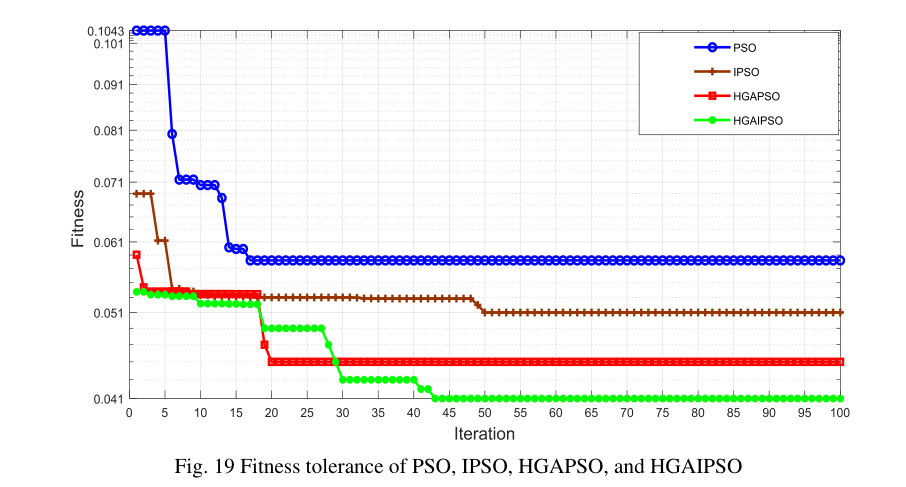
If you are interested in plot some like your Fig. 19, you could use the contents of
myBayesianAnalysis.Results.Sample and myBayesianAnalysis.Results.ForwardModel
(see Section 3.2 in the UQLab-Manual for Bayesian Inversion) to evaluate your fitness function. Here, you have to deal with the additional complications that in uq_Example_Inversion_08_Surrogate the default choice for the MCMC-scheme of UQLab is used, i.e. the Affine invariant ensemble algorithm (AIES). In this scheme, each “iteration value” is a vector of sample values. So, you would have to decide if you evaluate the fitness value at the average of the sample values, or the average/ the minima of the fitness values computed for all sample values.
But I fear you would not like the results since I expected that this value will somehow oscillate, since the algorithm is not working in the way you seem to expect.
You wrote ``
I am not sure, but if you refer here to the MCMC-algorithm used by UQLab for solving the inverse problem then I have to point out that this is not what this algorithm is designed to do. It is the aim of the different MCMC- algorithm used by UQLab to generate a set of samples reflecting the posterior density provided by Bayes’ Theorem, and this
posterior density combines the information on the unknown input parameter value
we get by combining the prior density and the observations.
Hence, it holds that the iterations points resulting from the algorithm will not converge to the unknown input parameter value, they are supposed to end up in cycles such that combining all iteration in one cycle creates a set of samples representing the posterior density.
Hence, if you would use the Metropolis–Hastings algorithm or the Adaptive Metropolis algorithm or Hamiltonian Monte Carlo algorithm or a similar one, the computed value of the fit-function should show strong/medium oscillations. For the
AIES scheme, i.e. the UQLab default choice, the oscillation may be medium/small, depending on your choice for the plotted values, see above.
Hence, if you want a plot like Fig. 19 with decreasing fitness values, you could plot
the minimal value over all fitness values up to the actual iteration, but this needs to be clearly pointed out in the description of the figure, since otherwise you would violate the rules of good scientific practice. Okay, this may be a plot of a well defined well-know quantity, but this depends on the situation.
Okay, now some finial remark: You seem to be interested to get some iterations scheme
showing some convergence such that you can use the limit value as approximation for the unknown input parameter value. If you are not interested to deal with the related uncertainty in form of a random density, using the MCMC-schemes formulated for Bayes Theorem may not be the best choice for you.
Greetings
Olaf