I am working with Bayesian Inversion, and I am pretty new to the topic. I have a similar question of this post.
I am performing some Bayesian Inversion from a model \mathcal{M} that uses 7 input variables (M=7) to produce 2 vectors (of dimension 7, N_\mathrm{out}=7…#confusionalert) as model output. As forward models, I use the previously computed PCEs. The outcomes are named HS and LS, respectively. As a reference
% 2. give forward model, in my case the PCE surrogates
ForwardModels(1).Model = PCE_HS;
ForwardModels(1).PMap = [1 2 3 4 5 6 7];
ForwardModels(2).Model = PCE_LS;
ForwardModels(2).PMap = [1 2 3 4 5 6 7];
bayesOpts.ForwardModel = ForwardModels;
I then perform the computation of the Bayesian problem, as in
% RUN IT FORREST
myBayesian_bothModels = uq_createAnalysis(bayesOpts);

% results are stored into myBayesian.Results. Generate good posterior sample with
uq_postProcessInversion(myBayesian_bothModels,'burnIn', 0.8,'pointEstimate',{'Mean','MAP'})
Now, I would like to extract the data point and the likelihood of the post-processed results. I had a look on UQ World, and so far, I could only find this solution (thank you @paulremo), but nothing regarding the likelihood values.
The inversion results show high multimodality of my model, highlighting different “areas” where the model parameters are calibrated. Therefore, I was thinking of adding a selection procedure of the results based on the likelihood values of each sampling point.
To be more precise, I would like to extract the values that color the results in shades of blue of the posterior distributions. @olaf.klein, do you know how to do this due to your past experience on the topic?
Again, I am pretty new to the topic, so I am probably mixing up some information here.
Have a look at the myBayesian_bothModels.Results.PostProc. structure. There should be a field .PostLogLikeliEval that contains the likelihood evaluations at the post-processed posterior sample points.
But be careful! In order to get the unnormalized posterior you will have to evaluate the posterior sample at the prior distribution and multiply those values with the likelihood evaluations stored in .PostLogLikeliEval.
On a more general note: Are you sure that the posterior is multimodal? Did you have a look at the trace plots of your MCMC sample (I assume you are using MCMC to solve the inverse problem)? Just to ensure that the multimodality is not a sampling artifact.
Hi Paul,
Thank you for your response. Eventually, I found out what I needed. I wanted to create my plotting script based on what UQlab produces with uq_display(myBayesian). In particular, I wanted to add the color information of the posterior distribution.
I had some spare time, dug into the codes, and noticed that the color is the normalized probability of the variables, not the likelihood. So I did solve my main question
This is also very interesting, although I do not know how to use this information. Do you know any good reference that I can read this?
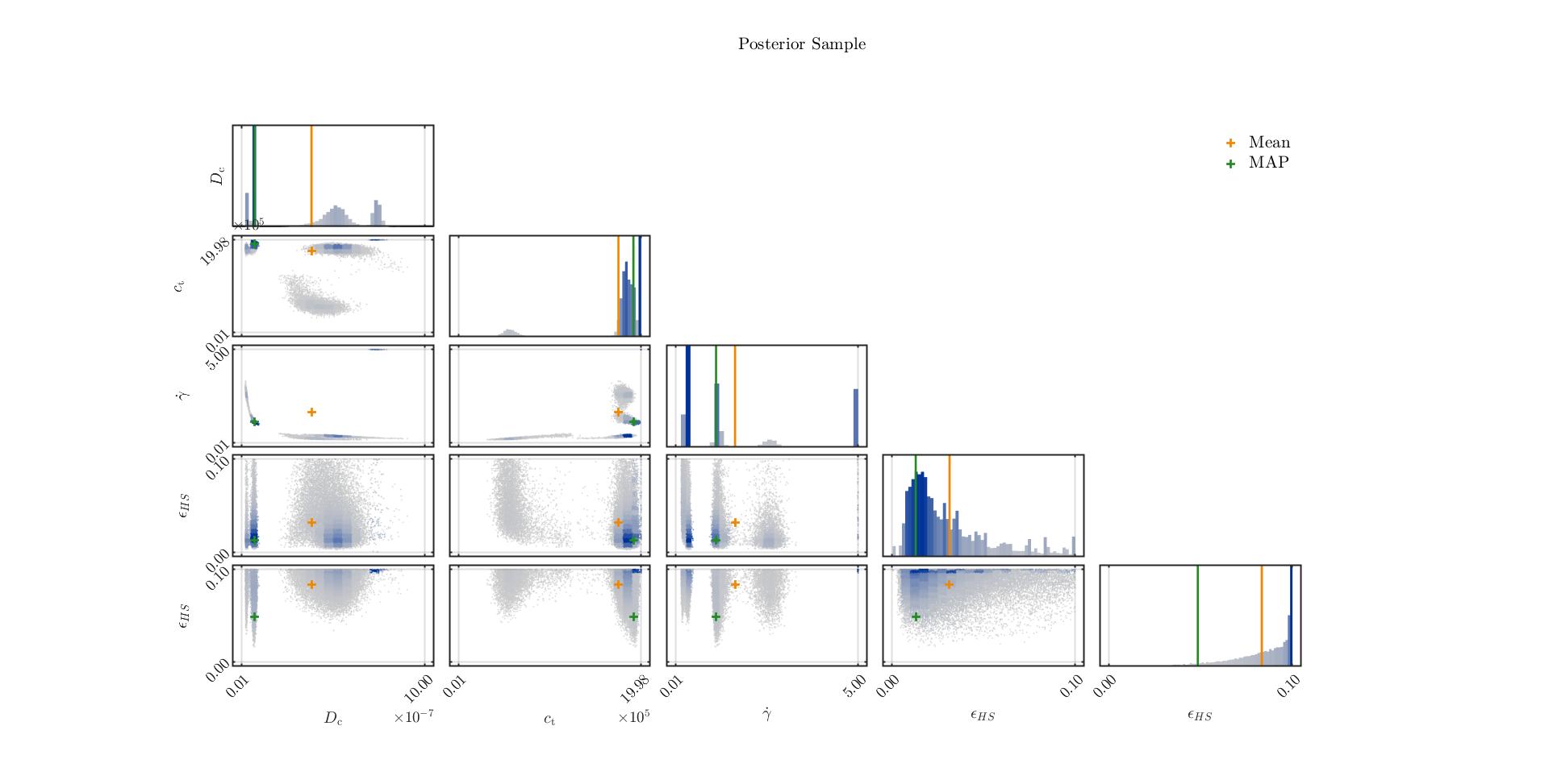
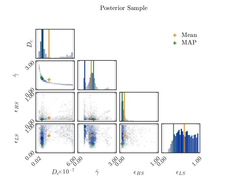
Mmm…I paste here my first preliminary result, i.e., the posterior distribution of 3 system variables and 2 discrepancy variances. Do not mind the names of these last two. I forgot to change them
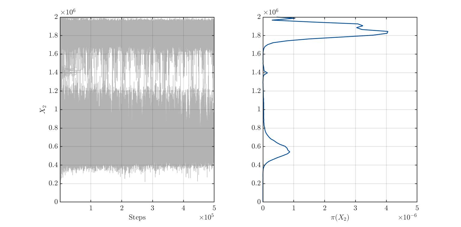
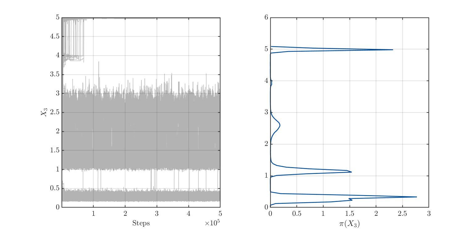
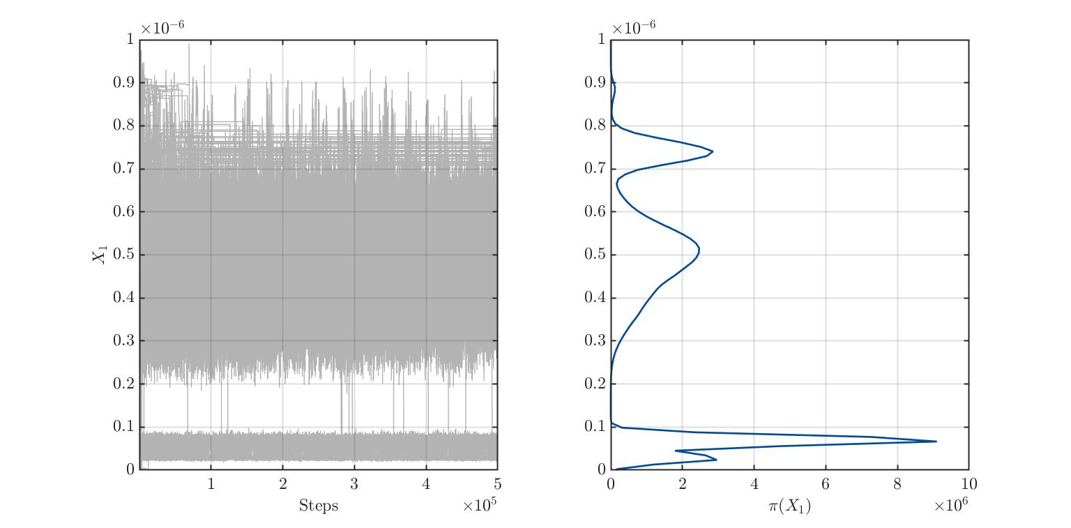
I am trying to find out the real distribution of 3 variables whose distribution is not known. The model is new and phenomenological. Therefore I got no information about the variables’ distributions. To find them out, I ran plenty of simulations with uniformly distributed variables and then performed a Bayesian inversion. I have the impression that there is multimodality. What do you think? I also paste the traces plots.
i.e., the product of the prior PDF \pi(\mathbf{x}) and the likelihood function \mathcal{L} divided by a normalization constant Z. To get the (unnormalized) posterior density you should thus multiply the likelihood values with the prior PDF.
Regarding your results, I see two problems:
Model specification: Which prior do you use? It looks like you use uniform priors for at least some parameters. Are they justified by your problem? Some parameters cluster at the upper and lower support which could mean that the uniform bounds are too narrow. And secondly, does the multimodality of the posterior make sense to you, i.e., can it be explained by the model?
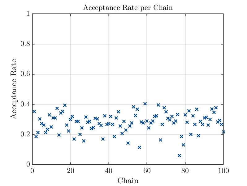
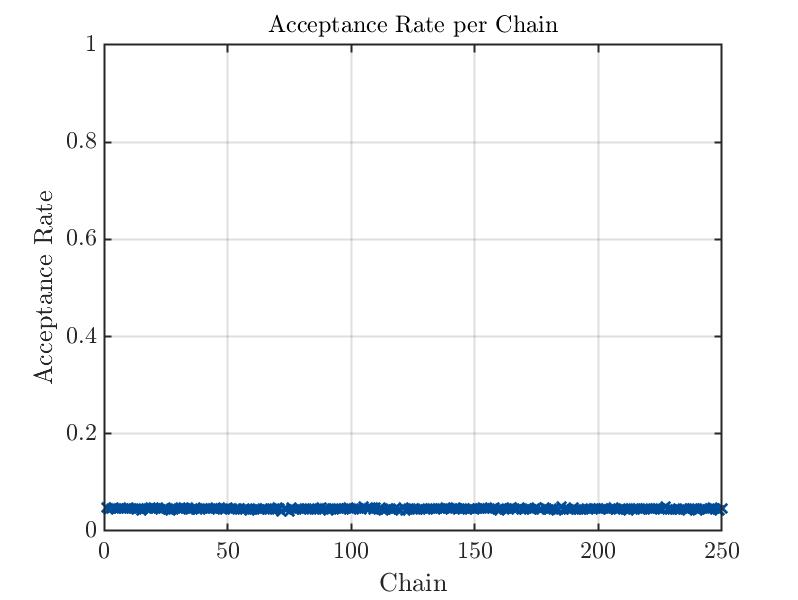
Sampler convergence: Which sampler do you use and how many burn-in iterations do you throw away? It looks like not all MCMC chains have reached their steady-state and for some chains the acceptance rate is extremely small. You should probably exclude the samples produced by those chains with a small acceptance rate from the posterior sample.
I have to investigate this more. For the moment, I have other questions, if I may
Yes, I use a uniform prior to my parameters. It is hard to say if such distribution is justified or not. As I mentioned, these are "made up"parameters. They are not measurable in the real world, so I am trying to determine their distribution with the Bayesian inversion. So I decided on a uniform prior because I have no information at all about their distribution. The model does not show limitations on their value, i.e., for any input given, the output exists. I am not sure if I answered you clearly
I noticed the clustering around the input bounds. So I am rerunning the model with different prior ranges. They are not really narrow. I think they are just misplaced.
the multimodality…probably can be explained by the model. Surely enough, I got to dig more into it.
I use the MH sampler. In these pictures, I left the default options. Therefore, I suppose that the burnIn is about 0.50.
I displayed the acceptance rate, which is extremely low, indicating wide prior distributions. Maybe in my second run, I will be luckier(?!). Anyway, how do I remove samples based on a small acceptance rate? Is it with badChains in uq_postProcessInversion(...)? I had a look at the .Results.Acceptance structure and found an acceptance rate for each chain. I suppose they refer to each chain. Therefore, it considers the acceptance rate of each chain in all the dimensions, right?
Overall I have to say that I noticed my results are not converging, or at least, I cannot trust them at this point. I also computed the Gelman-Rubin diagnostic and found out it is around 60. This means I am far away from the final solution, I suppose. What is still unclear to me is: should I increase the number of chains (currently 250) or increase the number of steps (currently 500000)?
Uniform priors are in fact pretty restrive when not chosen properly - they strictly constrain your parameter space to their bounds, so you have to be extra careful on choosing these bounds.
The MH sampler is quite fast, but it can be difficult to tune properly, i.e. choose a suitable proposal distribution. I suggest you run your problem with the affine invariant ensemble sampler (AIES) at least once. It is a bit slower, but is much less prone to miss-tuning. With this sampler, you could probably also reduce the number of steps !
Hi @paulremo,
Here I am. I got lost in Bayesian computations
Yeah, I noticed it. I reduced the ranges noticeably, and now I am more confident in what I see. Thank you for that.
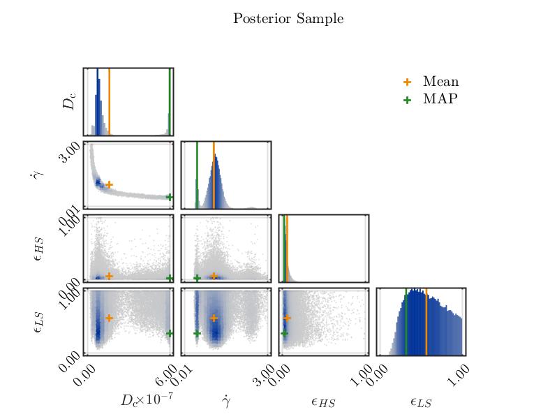
As of this, I did some experiments with the new ranges. I performed more model simulations, and now I decided to calibrate only 2 parameters of my 2 models, plus the discrepancies. I am comparing the 2 MCMC solvers, i.e., MH and AIES, but I am confused about what I see in the results.
Some running info
MH
% INPUT
bayesOpts.solver.MCMC.Steps = 500000; % number of iterations
bayesOpts.solver.MCMC.NChains = 250; % number of chains

%------------------- Solver
   Solution method:                               MCMC

   Algorithm:                                     MH
   Duration (HH:MM:SS):                           26:46:56
   Number of sample points:                       1.25e+08
AIES
% INPUT
bayesOpts.solver.MCMC.a = 2; % scalar for the AIES solver

%------------------- Solver
   Solution method:                               MCMC

   Algorithm:                                     AIES
   Duration (HH:MM:SS):                           00:19:07
   Number of sample points:                       3.00e+04
The AIES seems to be extremely faster than MH, contrary to what you said. So I am not sure if I am doing something extremely wrong here
Since the GR value approaches 1 for convergence of the algorithm, I assume that the MH performed better. +1 point for MH.
If I plot the convergence plots for my parameters, I see that the MH algorithm is more stable around one value for each parameter, which is why the GR diagnostic is better for MH. Is it correct?
The results are very similar, apart from the MAP point. But I wouldn’t care much for that since both solvers’ posterior distributions look the same. They are both able to detect the high correlation among the 2 parameters, which is fantastic. Due to the speed of AIES, I’d say, +1 point for AIES.
The results are very similar, as visible from the results printed above. I suppose the MH looks a bit better due to the larger number of iterations and chains. Which takes a long computing time…therefore +1 to AIES
Conclusions
The match concludes 3 to 1 for AIES. The question is, am I correct?
Thank you for your help and patience in reading all of this
The comparison you are making is not really fair because with AIES you produced “only” 3\cdot 10^4 sample points, while you produced 1.25\cdot 10^8 with MH. That’s an increase by 4 orders of magnitude! The remark I made about the speed has to take the number of produced samples into account. If you correct for that, you can clearly see that AIES is much slower per produced sample.
I would not worry too much about the acceptance rate, however, the Gelman-Rubin MPSRF is too large for AIES.
Looking at your results, it seems to me like MH has run for too long, while AIES could use a few more iterations. From a practical point of view, it seems that both algorithms do a decent job at sampling the posterior distribution, so I would pick the faster MH algorithm. It should be able to solve your problem efficiently by reducing the number of iterations by one or two orders of magnitude. This will cut down the sampling time to somewhere between 10 minutes and 1 hour.
Hi Paul,
Thank you for this. I was expecting your comment already. I dug in the user manual, and I noticed that I could also change the number of steps and chains with the AIES solver. Somehow I thought this was locked to default and that the only variable for AIES was the a scalar.
Thank you for your help!
It was a good step forward

 ), but nothing regarding the likelihood values.