Reliability analysis with AKMCS: some doubts and question on a specific application

Hello everybody.
I have some doubts regarding the functioning of the reliability analysis module for my particular problem. Here are the details.

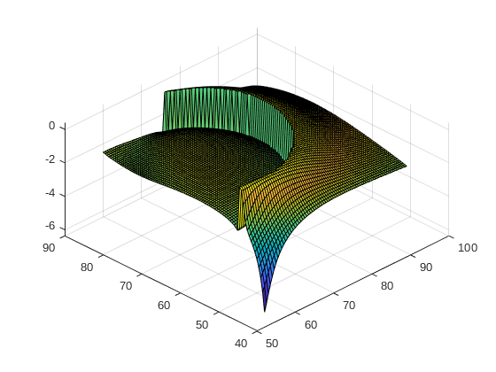
I am using the reliability analysis of UQlab on a model with input space dimension 2. I decided to compare the AKMCS method with the MC method. This one will be considered as a benchmark for the problem.
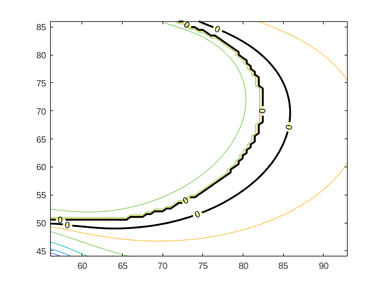
I set the MC module with the comparison operator, I set the model, and I start the module simulation. The simulation stops with 10^5 runs, and I get my benchmark simulation. The areas of safe and fail are easily visible if I type the “uq_display” command.

Then, I set the AKMCS with Kriging metamodel in the following way: I choose the correlation family, the comparison operator for the limit state function, indicate the initial input experimental design, set the max added ED at 500 and set the convergence function with StopU (I also tried with StopPf).

The AKMCS with PCK metamodel has been set with the same properties. I run both of them, but I am not satisfied with the results I get. Here, they are listed:

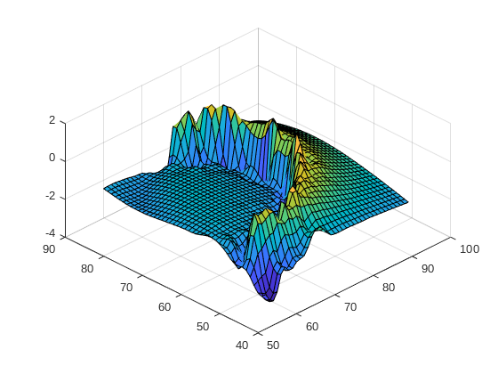
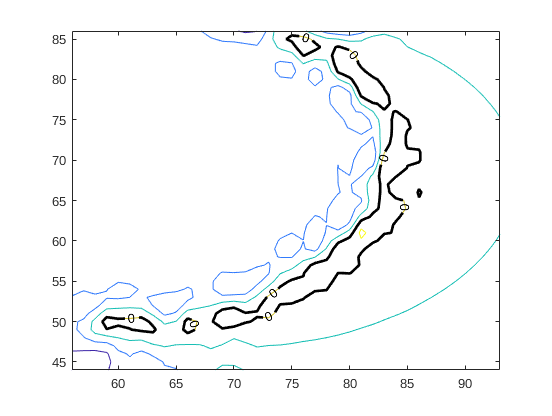
  1. I do not get the convergence for both method AKMCS. They reach the 500th simulation without converging (for both methods and convergence functions). When I display my reliability analysis, I can see that the module has found most of the limit state function, but the confidence interval of the probability of failure is far away to converge;

  2. the simulation time of both AKMCS is 10^1 or 10^2 times bigger than the MC one. This problem is the main problem of my simulation because it should result in a less computational effort, but it is not the case if I look at the simulation time.

I think, and I am afraid that the main issue is that my model is “too easy” for this application and therefore, AKMCS makes just everything more complicated. My model is deterministic.

In case there are some details missing, I would provide you with more information.
Thank you in advance for any help

Best,
Gian Marco

Hi @giansteve, welcome to UQWorld!

To start, how big is your 2-parameter model? Is it possible to put the code here in the forum? It will certainly help in reproducing your problem.

Hi @damarginal, thank you :slight_smile:

Here I paste my deterministic model. The output is a structure of parameter of the best fit ellipse from a set of existing points, to which one random point in the x-y plane is added.

function ellipse = GM_ellipseDC(DCS, X, Eplot)
% Computation of the best fit ellipse by using least square algorithm.
% INPUT:
% - DCS: points of the existing geometry;
% - X: new point to add to the geometry;
% - Eplot: handle for plot
%
% OUTPUT:
% - ellipse: structure with ellipse parameters.
%
% REFERENCE:
% Gal, O., (2003). fit_ellipse.m
%
% ========================================================================

[a,b,phi,x0,y0,x0phi,y0phi,L,l] = deal([],[],[],[],[],[],[],[],[]);

% Getting the right points of the cross section
TL = DCS.ContTL;

% Weights of points
wTL = 1;
wX = 1;
% rotation tollerance
toll = 1E-04;

% transform the input in columns
% x = [repmat(TL(:,1),wTL,1);repmat(X(:,1),wX,1)];
% y = [repmat(TL(:,2),wTL,1);repmat(X(:,2),wX,1)];
x = [TL(:,1);X(:,1)];
y = [TL(:,2);X(:,2)];

% compute mean and standardize the input
xMean = mean(x);
yMean = mean(y);

x = x - xMean;
y = y - yMean;

% Estimation of Phi angle
lastwarn = '';
Coeff = [x.^2 x.*y y.^2 x y];
Coeff = sum(Coeff,1)/(Coeff'*Coeff);
% check for warnings
if ~isempty( lastwarn )
    disp('Error in inversion matrix' );
    ellipse = [];
    return
end

F = -1;
[A,B,C,D,E] = deal(Coeff(1),Coeff(2),Coeff(3),Coeff(4),Coeff(5));

% tilt angle
if min(abs(B/A),abs(B/C)) > toll
    phi = 1/2 * atan( B/(C-A) );
    c = cos(phi);
    s = sin(phi);
    % coefficients: c stands for conic equation
    [A,B,C,D,E] = deal(A*c^2 - B*c*s + C*s^2,0,A*s^2 + B*c*s + C*c^2,...
        D*c - E*s,D*s + E*c);
    [xMean,yMean] = deal(c*xMean-s*yMean, s*xMean+c*yMean);
else
    phi = 0;
    c = cos(phi);
    s = sin(phi);
end

% Conic eqn = ellipse ?
test = A*C;
if (test == 0)
    ellipse = struct( ...
        'a',a,...
        'b',b,...
        'phi',phi,...
        'x0',x0,...
        'y0',y0,...
        'x0phi',x0phi,...
        'y0phi',y0phi,...
        'L',L,...
        'l',l,...
        'obj','Parabola');
elseif (test < 0)
    ellipse = struct( ...
        'a',a,...
        'b',b,...
        'phi',phi,...
        'x0',x0,...
        'y0',y0,...
        'x0phi',x0phi,...
        'y0phi',y0phi,...
        'L',L,...
        'l',l,...
        'obj','Hyperbole');
end

% center of the ellipse
x0 = xMean - D/(2*A);
y0 = yMean - E/(2*C);
% square completion method
Fcc = -F + D^2/(4*A) + E^2/(4*C);

% semiaxes
a = sqrt(abs(Fcc/A));
b = sqrt(abs(Fcc/C));
% long and short axes
L = max(a,b)*2;
l = min(a,b)*2;

% rotate the axes backwards to find the center point of TILTED ellipse
R           = [c s; -s c];
Pphi        = R * [x0;y0];
x0phi       = Pphi(1);
y0phi       = Pphi(2);

% response
ellipse = struct( ...
    'a',a,...
    'b',b,...
    'phi',phi,...
    'x0',x0,...
    'y0',y0,...
    'x0phi',x0phi,...
    'y0phi',y0phi,...
    'L',L,...
    'l',l);

% plot?
if nargin>2 && Eplot ~= 0
    if Eplot == 3
        alpha = linspace(0,2*pi);
        ellipse_x = x0 + a*cos(alpha);
        ellipse_y = y0 + b*sin(alpha);
        rotEllipse = R * [ellipse_x;ellipse_y];
        
        plot(rotEllipse(1,:),rotEllipse(2,:),'r-','LineWidth',2.5);
    else
        alpha = linspace(0,2*pi);
        ellipse_x = x0 + a*cos(alpha);
        ellipse_y = y0 + b*sin(alpha);
        rotEllipse = R * [ellipse_x;ellipse_y];
        
        plot(rotEllipse(1,:),rotEllipse(2,:),'b:');
    end
end

end

I tried to reduce the code length as much as possible. I hope it is still good enough.
My MATLAB version is 2019a; UQlab version is 1.2.0.

Let me know if something is not clear.

Best, Gian

Hi Gian, sorry that I was not complete on my first suggestion about reproducing the problem. At this point, unfortunately, it still hard to reproduce your problem.

Can you let us know more about your analysis script as well. It should include:

  • the probabilistic input model
  • all the options for the reliability analysis you set, e.g., What is the limit state function? You also mention about using the comparison operator, but how is it defined? Using which value of threshold?
  • additional input of the model if it’s not part of the probabilistic input model (e.g., DCS?)

Thanks!

Hi. Ok, sorry that I was not complete as well. So, I will list the information you asked for:

  • the probabilistic input model is composed of 2 uniform distributed RVs. They represent the coordinate in the xy plane of a point. This point is the input X in the deterministic model that I posted.
  • the input DCS represents a set of points extracted from a picture. So, the input DCS and the random point X are added at each iteration, and together they form an ellipse E_D in the xy plane.
  • the final ellipse is then compared with another ellipse that is considered fixed and known, let’s call it E_H. In other words, the set of points DCS, together with the random point X, must recreate a geometry E_D that has the same property of the initial geometry E_H.
  • the options for the reliability analysis are:
    • the limit state function operator is <
    • the limit state function threshold is left as default, so 0
    • the degree of the polynomial for the PCK case is left as default, but I started with degree 2
    • the initial experimental design X is computed from uq_getSample(UQInput,N,'mc'), where UQInput is the input model, N is the number of samples I want to get (usually fixed at 100).
    • the convergence criterium is based on stopU.
    • other options are not changed and left as default

This should be all that is needed. I will provide more if needed.
Thank you a lot in advance

Best, Gian

Hi Gian, thanks for the description. To complete your problem specification, some additional info is still needed:

  • What are the bounds for the uniform distributed RV?
  • Do you have an example of a DCS from a picture that you used for the problematic analysis? I can see that it’s structure. Note: you can also attach your file here in the forum if it’s not too big (If it’s too big, we’ll find another way :slight_smile:) .
  • What is the reference ellipse E_H you used?
  • The output of your posted model is itself a structure (with the properties of the ellipse), but what is being evaluated in the limit state function that gives the fail/safe status? I suppose, as you said, it is compared with a known ellipse. But how are they actually compared?

Our first goal is to run and reproduce your problem (I run this, I expect this, but instead, I got this) here in our workstation. So don’t hesitate to post the analysis script and/or attach files (<4MB) that might be helpful for doing this.

Thanks!

Hi Damar.
Perfect. So, I am now working on making the scripts more readable and on making everything running as smooth as possible.
All the Matlab scripts and the figure have a dimension of 3,47 MB. I suppose that I can attach them here, right?

I will post as soon as I can :slight_smile:

Thank you and speak soon
Gian

Hi Damar.
Here I attach the ZIP file with all the code you may need to run the analysis. The main file is called “Main_RA_FINAL.m”.

UQWorldCodesCheck.zip (11.1 KB)

To your questions:

  1. the structure DCS defines the bounds of the uniform RVs. In this structure, there is DCS.DD who represent the contour plot of my image, DCS.TL who is the “good data” that I want to augment with the point X (my random vector), and DCS.FL who represent the “bad data” that I do not want to keep in my simulation. Anyhow, this last set of points DCS.FL defines the bounds of the uniform RVs through the variable maskk. In other words, the bounded region is like an area where to start the research;
  2. the example of the DCS image you will find it in the ZIP file;
  3. the reference ellipse is computed with the Matlab script GM_ellipse.m from the set of points in the variable HCS.ContHR.
  4. the limit state is the value 0. In the script GM_model.m I compute the ellipse of the point (3), then I compute the ellipse that results from the DCS.TL points + the random vector X with the code GM_ellipseDC.m. From both ellipses, then I compute a result that allows me to compare them. You will find the formulas in the GM_model.m at lines 26,67, and 68.

Let me know if something is not clear. I always find it very hard to explain codes with standard text.
Thank you a lot :slight_smile:
Best, Gian

Okay, let me have a look at them first.

Hi @giansteve, I’ve had a look at your problem and I think I manage to reproduce it.
To come back first to your initial remarks/questions:

  1. There are cases in which AK-MCS (or APCK-MCS) performs worse in terms of wall time, especially when the limit state function is very fast to evaluate. Remember that constructing a Kriging (or PCK) metamodel of the limit state function at each enrichment step incurs an additional overhead cost. This cost might not worth it for a very fast model. In your case, that is indeed the case.

    When comparing reliability methods using benchmark problems of which the models are often cheap to evaluate, the measure of computational effort is usually the number of limit state function evaluations or calls and not the wall time.

  2. Regarding your question about the convergence of AK-MCS, I think you raised a good point. The model might be relatively fast to evaluate, but contrary to what you might think, I don’t think it is easy.

You might already be aware of this, but I put a figure of your limit state function below. As you can see it is a discontinuous function and that the safe region lies near the discontinuity.

lsf_full lsf_full_contour

I think Kriging, at least the one currently available in UQLab, would have problem reconstructing such a surface.

lsf_kriging lsf_kriging_contour

Recall that one of the convergence measures used to stop the enrichment iteration is the convergence of failure probability as measured by the difference between the lower and upper bounds (p. 17 of the Reliability User Manual). The problem is that the standard deviation of the Kriging approximation used to construct the upper and lower bounds tends to be very large and it converges very slowly at each enrichment step; it seems that the enrichment does not bring much to improve this convergence.

I’m not sure, however, how you can improve AK-MCS for this particular case, maybe @Xujia or @moustapha can help?

2 Likes

Hi @damarginal, thank you so much for your response and sorry for the delay of mine.

I noticed that the number of simulation is way lower for the 2 AKMCS cases, but still they do not reach convergence. May I ask you if in your simulation you get to convergence? And if yes, how many runs did the metamodel do?

At the moment I am trying to give different geometries as input to check how the system behaves. At the same time I am trying slightly differents models that produce different limit state functions, but the problem of slow convergence still exist.

I will let you know if I find something special…
By the way, thank you for the time you put in this. At least now I know that it is not only me seeing weird results.

I will post an update as soon as I get some.
Best
Gian

No problem!

No, my AKMCS run did not converge either with initial points of 500 and enrichment points of 500. I am not sure though that it will ever converge with any reasonable numbers of enrichment points in the sense of the applied convergence criteria. Because, in my opinion, this discontinuity in the limit state function is really a problem for Kriging or PC-Kriging, especially in terms of the associated standard deviation used in the criteria. I guess you would need lots of points to capture that discontinuity with Kriging.

Now of course you would also notice that the estimate of P_f (the blue line in the plot by uq_display) is stable across enrichment (but with a super wide convergence band). This number won’t be too different from the estimate from direct MCS, I suppose.

I haven’t really check what’s actually inside your model, but if we refer to the figure you notice that there’s this cliff near the safe region. Do you think it’s possible for you to shift that region up? That is, to make the difference in the level not as dramatic like that. It might help Kriging in reconstructing the surface.

Moreover, maybe I didn’t get it the first time, but are you using AK-MCS for this case solely for benchmarking purpose (with other methods also)? With a fast model like this one, you can afford to use more direct approach, right? Or maybe you’re doing something else?

Thanks!

Hi.
I will answer you question:

  • Regarding the cliff close to the limit state function: do you mean that the SAFE/FAIL criteria shoul be not as restrictive as it is, in terms of the result of the metamodel? So, does that means that I would need to have different limit state functions? If this is the case, I do not think I know how to do so…

  • I am using AKMCS because I would like to use this method also for other applications, and not only for civil/mechanical engineering, where it is best known. In this particular case, I am trying AKMCS for an image reconstruction. Other methods could be applied and may be faster, but, it is my intent to use PCE (or PCK here) since my work is mainly based on it.

Everything started when I started reading about the AKMCS method and I wanted to test it for the research of points for image reconstruction or augmentation. In theory it works, but I think it is just too slow given the overhead problem…

Best,
Gian

Hi @giansteve, thanks for the answers!

  • I have no idea either, not a concrete one at least. But I’ll have a look again at the model and try to understand it better later.
  • Aha okay! I am actually very interested in your application :slight_smile: (artery and all), maybe others here are too… So how would you use the probability of failure in your case? Image classification?

Hi @damarginal, sorry for the delay: this application is driving me crazy :slight_smile:

I tried different models to check out if it is possible to make the limit state function not discontinuos, and to delete or “to smooth” the cliff close to the safe region. I am still working on it, and I may have found a solution.

Furthermore, I realized that SVM for Classification does exactly what I need in 1/100 of the time that AKMCS needs. This discovery left me a bit sad I have to say, but never say never…

Regarding the application, exactly! It is an idea I had for recovering geometries from a dataset that is “damaged”. In my case, I have a healthy and a diseased condition of a cross-section. What I want is to go back to the healthy condition from a diseased one collecting information from other pictures. These other pictures, will refere as the knowledge that carries my safe threshold. The probability of failure at the moment is only a way to satisfy convergence, so it has no particular meaning. In the future, so when the actual problem is solved, my idea is to have more reference images that will represent a statistical information about my safe treshold. So the probability of failure would be a statistics on the result.

I hope it is clear enough, I tried to recap as much as possible without deepening to much into details. Of course, I will provide as much information as needed if that is the case.

Best,
Gian

Hi @giansteve,

Got it!

By the way, the recent work of @moustapha is actually in this direction. But this work is not part of UQLab release. The next time he drops by UQWorld, he might be able to help you. In the meantime, I encourage you to go through his recent presentation, to get the main idea; you might be able to find your own way in the process.

Hi Damar,

Thank you so much for sharing the presentation of Mr Moustafa. It is incredibly similar, at least the plots and the discontinuity problem.
I think I will contact him for further question :slight_smile: Thank you very much for your help. This project was quite ambitious since the beginning and became even more weird in time, but I will try to figure something out.

Hi @giansteve,

I tried this afternoon to run your model through the algorithm we developed in the conference paper, @damarginal mentioned earlier. I could get good prediction capability by combining SVM and Kriging. However, the approach works only given that we can tell a priori to which region does a given sample of the experimental design belongs. This can be done manually in this specific case. Do you have any automated criterion or additional information that would allow you to discriminate these two distinct regions of the space ?

In general, AK-MCS is clearly not a solution for your model. As you mentioned, you could build ad-hoc an SVM model and use this in a Monte Carlo analysis. However if you still want to have predictive capabilities, you may need to do what we did in the paper, i.e. build two local models instead of a global one.

Cheers,
Moustapha