Polynomial chaos expansion with vine copula input

Hi everyone,

I am studying PCE and I have encountered a problem that troubles me quite a while. I’d appreciate it if I can get any help or advise from you.

I read from manual that UQLab supports copula now, so I try it on the example provided in section ‘Calculation strategies’. I would like to know what would happen if we still assume the inputs are independent when the actual inputs are in vine structure. Or how much impact copula will have onto the PCE metamodel.

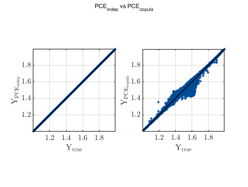
So I create another input with copula structure and run the example again. This time I get two PCE metamodels, one is based on independent inputs while the other is based on inputs with C-vine structure. The marginals of two types of inputs are the same. The only difference is the copula type. As done in the example, I produce scatter plots of the metamodel vs. the true response. However, I cannot get the desired results.

I am wondering what is the appropriate way to construct PCE based on inputs that have copula structure and how to debug in this situation.

Thanks for your time.

Best

3 Likes

Hi Charol, welcome to UQWorld! :slight_smile:

That’s a very interesting question! When PCE are used, most of the time it is assumed that the input variables are independent. But what to do if they are dependent? There are several options:

  • Ignore that there are dependencies and build a PCE with basis polynomials that are orthonormal wrt. the input marginals.
  • Transform the input into independent variables (isoprobabilistic transform), then build a PCE on these independent variables.
  • Build arbitrary PCE with basis polynomials that are orthonormal wrt. the (dependent) probability density function.

The first two approaches have been compared in the recent paper
Torre, Marelli, Embrechts, Sudret (2019): Data-driven PCE for machine learning regression
under the names aPCEonX (first approach) and lPCEonZ (second approach). They find that the first approach aPCEonX yields better pointwise estimates than lPCEonZ and explain this with the non-linear mapping that is needed to transform the input into independent variables, which can make it difficult to approximate the resulting model by PCE.

For the third approach, there exists an analytical formula for the orthonormal basis polynomials functions, but investigations of Emiliano (@torree) have shown that this approach does not perform well in comparison with the others. I faintly remember that there is another recent publication on PCE for dependent inputs, maybe @torree knows more?

By default, when you use UQLab to construct a PCE for dependent inputs, the second approach is used (transformation to standard marginals and independent copula using uq_GeneralIsopTransform).

Now to your second question

You describe that you compared PCE metamodelling for the Ishigami function with independent and with dependent inputs.

What are the desired results that you expected to see, and what are you seeing instead? Could you maybe provide us with the plots that surprised you, and the copula that you used? It might be that you are observing precisely this issue with the highly non-linear mapping to independent variables that Torre et. al. describe in their paper.


By the way, in case you haven’t seen it yet, here is a nice post by Emiliano on the importance of using the right dependence structure for your inputs when doing UQ.

1 Like

Hi Nora,

Thank you for your reply.

Blockquote
The first two approaches have been compared in the recent paper
Torre, Marelli, Embrechts, Sudret (2019): Data-driven PCE for machine learning regression
under the names aPCEonX (first approach) and lPCEonZ (second approach).

Very interesting paper. It opens a new world for me. So aPCEonX outperforms lPCEonZ on pointwise estimation while lPCEonZ yields better statistical estimates. I assume these statistical estimates come from coefficients of PCE we constructed, right? If so, does that mean that the statistical estimates obtained from PCE coefficients are different from the ones calculated from empirical results (attained from same PCE) when it comes to highly non-linear copula?

Blockquote
What are the desired results that you expected to see, and what are you seeing instead?

After constructing PCE, I believe we can employ this PCE model as a surrogate model for original one. Since the real inputs are non-linear related. I thought lPCEonZ would provide better empirical result for both pointwise prediction and statistical estimates.

Blockquote
Could you maybe provide us with the plots that surprised you, and the copula that you used?
Blockquote

I am not sure if this is normal according to that issue.

The copula parameters are:
Type = ‘CVine’
Families = {‘t’, ‘Frank’, ‘Clayton’};
Parameters = {[0.5, 1], 0.5, 1.5};

Thank you again for your detailed explanation.

Hi Charol,

Yes, aPCEonX outperforms lPCEonZ regarding pointwise estimation. It is not clear in general which one yields better statistical estimates: For the Ishigami function, aPCEonX is better; for the horizontal truss, they perform similarly except for the standard deviation, where lPCEonZ performs slightly better. In general, if the pointwise convergence is good, then also the moments will be estimated well.

No, they are computed by propagating a large set of samples from the input distribution through the PCE models (Torre et. al. 2019, Section 3.1). It would not be possible to use the coefficients of aPCEonX to compute the moments, since in this case the basis functions are not orthonormal wrt the input distribution. For lPCEonZ it should be possible, but maybe the authors wanted to use the same computation method for both approaches to be comparable.

Regarding your plots: Yes, this can happen. The Ishigami function is very sparse in the Legendre polynomial basis. If you use the approach lPCEonZ, what you are actually surrogating is the Ishigami function combined with the inverse of the transformation from the dependent input X to independent standard variables Z:

\mathcal{M}_\text{lPCEonZ}(Z) = \text{Ishigami}(T^{-1}(Z))

The transformation T from dependent to independent standard variables can be highly nonlinear. It is possible that \mathcal{M}_\text{lPCEonZ} cannot be well approximated by polynomials anymore. It is also possible that \mathcal{M}_\text{lPCEonZ} is not sparse anymore in the PCE basis. This is not so critical when we have enough experimental design points available (i.e., many more points than unknown coefficients), since in this case we can use least-squares, but if we want to use sparse regression methods like LARS with few design points, non-sparseness can deteriorate the solution a lot.

Another view on this is the following: PCE work so well because engineering models are often smooth, close to polynomial, and follow the sparsity-of-effects principle (a heuristic saying that the most important terms have low interaction order). The engineering model does not know or care about what distribution the inputs have, it simply follows from the laws of physics (and some simplifications). If we now introduce the transformation from dependent to independent input variables, we change the model structure and might lose all these favourable properties. Imagine that for the same model, we try out several inputs, each with a different dependence structure. With the approach lPCEonZ, we would have to approximate totally different models each time, even though the physical mechanism is the same in all cases! This shows that also conceptually the approach aPCEonX might be more meaningful.

There are more open questions on this topic, e.g., which distribution should the training set be sampled from - from the dependent input distribution or from the product of the input marginals, corresponding to the distribution orthogonal to the aPCEonX basis functions?

If you come across interesting publications in this direction (PCE with dependent input variables), please share them with us! :relaxed:

1 Like