PCE error in UQlab vs chaospy

Aep93 · October 28, 2024, 4:18am

Hello all,
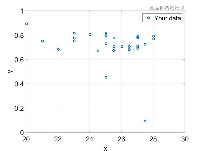
I am implementing PCE in chaospy with Python and Uqlab with MATLAB, but I get different outcomes. In Python, the LOO is around 2%, but in MATLAB, it is 100%. I am wondering what is wrong with the UQLab MATLAB code? Here is my code:
MATLAB code:

clear
uqlab
data = [
    25.532, 0.776;
    27.487, 0.724;
    27.032, 0.788;
    25.512, 0.673;
    27.489, 0.092;
    25.032, 0.453;
    26.498, 0.706;
    23.032, 0.775;
    27.032, 0.702;
    25.532, 0.705;
    27.032, 0.691;
    24.532, 0.669;
    25.032, 0.794;
    27.032, 0.709;
    26.498, 0.681;
    25.032, 0.807;
    24.032, 0.805;
    28.032, 0.791;
    22.032, 0.682;
    26.032, 0.705;
    23.032, 0.751;
    21.032, 0.750;
    25.032, 0.816;
    23.032, 0.815;
    26.498, 0.679;
    25.032, 0.729;
    20.032, 0.892;
    27.032, 0.778;
    28.032, 0.768
];

% Use only the first and last columns
x = data(:, 1);
y = data(:, 2);

% Define the input marginals
InputOpts.Marginals(1).Name = 'X1';
InputOpts.Marginals(1).Type = 'Gaussian';
InputOpts.Marginals(1).Parameters = [mean(x), std(x)];

myInput = uq_createInput(InputOpts);

% Define the PCE metamodel
MetaOpts.Type = 'Metamodel';
MetaOpts.MetaType = 'PCE';
MetaOpts.ExpDesign.X = x;
MetaOpts.ExpDesign.Y = y;
MetaOpts.Degree = 2; % Ensure the same polynomial degree
MetaOpts.TruncOptions.MaxInteraction = 1; % Ensure the same truncation options

myPCE = uq_createModel(MetaOpts);

uq_print(myPCE);

##########################
Python code:

import numpy as np
import chaospy as cp
from sklearn.linear_model import LinearRegression
from sklearn.model_selection import LeaveOneOut
from sklearn.metrics import mean_squared_error

# Provided data
data = np.array([
    [25.532, 0.776],
    [27.487, 0.724],
    [27.032, 0.788],
    [25.512, 0.673],
    [27.489, 0.092],
    [25.032, 0.453],
    [26.498, 0.706],
    [23.032, 0.775],
    [27.032, 0.702],
    [25.532, 0.705],
    [27.032, 0.691],
    [24.532, 0.669],
    [25.032, 0.794],
    [27.032, 0.709],
    [26.498, 0.681],
    [25.032, 0.807],
    [24.032, 0.805],
    [28.032, 0.791],
    [22.032, 0.682],
    [26.032, 0.705],
    [23.032, 0.751],
    [21.032, 0.750],
    [25.032, 0.816],
    [23.032, 0.815],
    [26.498, 0.679],
    [25.032, 0.729],
    [20.032, 0.892],
    [27.032, 0.778],
    [28.032, 0.768]
])

# Split input and output data
X = data[:, 0].reshape(-1, 1)
y = data[:, 1]

# Define the distribution of the input variable (assuming normal distribution)
mean = np.mean(X)
std = np.std(X)
distribution = cp.Normal(mean, std)

# Create a joint distribution
joint_dist = cp.J(distribution)

# Define the polynomial expansion
polynomial_expansion = cp.generate_expansion(2, joint_dist)

# Evaluate the polynomial expansion at the data points
X_poly = cp.call(polynomial_expansion, X.T).T

# Initialize Leave-One-Out cross-validator
loo = LeaveOneOut()

# Initialize lists to store results
y_true = []
y_pred = []

# Perform Leave-One-Out cross-validation
for train_index, test_index in loo.split(X_poly):
    X_train, X_test = X_poly[train_index], X_poly[test_index]
    y_train, y_test = y[train_index], y[test_index]
    
    # Train the model
    model = LinearRegression()
    model.fit(X_train, y_train)
    
    # Predict the output
    y_pred.append(model.predict(X_test)[0])
    y_true.append(y_test[0])

# Calculate accuracy (mean squared error)
mse = mean_squared_error(y_true, y_pred)
accuracy = 1 - mse

print(f"Leave-One-Out Mean Squared Error: {mse}")
print(f"Accuracy: {accuracy}")

styfen.schaer · October 28, 2024, 10:08am

Dear @Aep93

They both perform equally poorly. You can plot the actual output against the predicted output to see this clearly. The reason why the Python code gives a good LOO error is that the error is not normalized. UQLab uses a normalized LOO, as explained in the manual:

Best regards
Styfen

Aep93 · October 28, 2024, 12:03pm

Thank you for your response @styfen.schaer.
So, I am wondering why my PCE is performing so poor even with only one input parameter. Do you have any suggestions that I can implement to increase its accuracy?

styfen.schaer · October 28, 2024, 2:31pm

There are several reasons why a PCE model may not yield good results. Just to name a few:

The explanatory power of the PCE model can be insufficient, possibly due to a degree that is too low.
The input variables might be insufficient to explain the output, meaning there could be missing factors that are not included in the inputs.
The model may suffer from overfitting if the polynomial degree is too high
If the input data has significant noise, the PCE model may struggle to generalize well

Based on the very limited information available to me (and also based on your other topic), I tend to think that point number two is a likely reason. What is that data you have and how did you obtain it?

bsudret · October 29, 2024, 5:14pm

Thank you @styfen.schaer for your answers already.

In the current case, it’s easy to see that the data shows inconsistencies. If there is a single input, then the points can be plotted in the (x,y) plane, and should show a curve that we then try to approximate with a polynomial.

The provided data points are shown in the figure above: there is obviously no structure, meaning that:

either the x’s don’t correspond one-to-one to the y’s
the y’s are actually obtained as a function of many more input, say y={\mathcal{M}}(x_1, x_2, \dots, x_n) and you only provided the data set of (x_1, y).

In any case, assuming you change the data, you should add to your UQLab options:

MetaOpts.Method = 'LARS';
MetaOpts.Degree = 2:15;

to use a sparse solver (LARS), and automatically check various maximal degrees for the polynomial basis.

Best regards
Bruno

Aep93 · November 11, 2024, 12:36am

Thank you @bsudret and @styfen.schaer for your helpful explanations.

I have another question related to this. I noticed something unusual:

I manually calculate the leave-one-out error as follows:

Create n PCE models, where in each model, one data point is removed from the full training dataset. For each model, I then train the PCE and calculate the absolute percentage error (APE):

MAPE=abs(y_true - y_pred)/y_true

After calculating the APE for each of the n models, I compute the average of all the APE values (MAPE) to obtain the leave-one-out error.

The leave-one-out error I calculate manually using the approach above seems reasonable (around 5%). However, the leave-one-out error computed by UQLab (via myPCE.Error.LOO) is significantly larger (around 90%).

I reviewed the UQLab manual and looked into how the leave-one-out error is calculated in UQLab. Now I’m uncertain whether I should conclude that my model does not generalize well because the LOO error calculated by UQLab is much higher, or whether the model is actually performing well because the manually calculated MAPE error is relatively low.

As an engineer, the approach I mentioned earlier is the method that I, along with many others in our field, have always used to calculate the leave-one-out MAPE error and validate models. However, UQLab’s approach to leave-one-out error is completely new to me. I’m wondering: can the PCE model developed with UQLab be validated solely using the LOO error reported by UQLab, or are other common validation metrics (such as the MAPE I mentioned earlier) considered reliable?