Dear UQLab team,
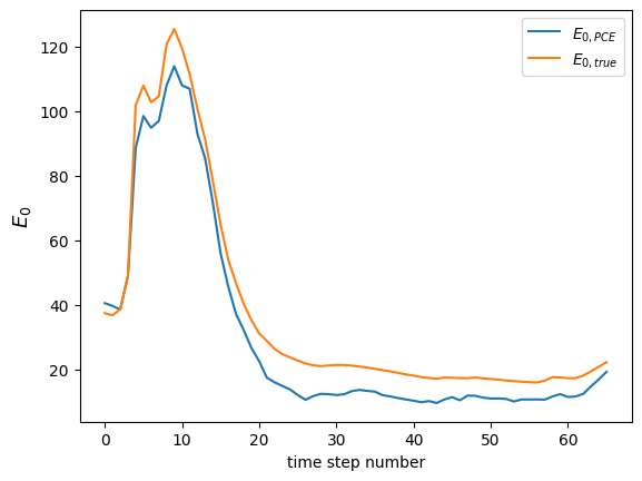
I am trying to run a PCE based sensitivity analysis of a hydrogeophysical model (the output of the model is a time series of geophysical signals at Nt = 66 time steps).
Here is a quick description of my problem and the experimental design :
- Problem dimensionality : 22 parameters
- Experimental design : Nsamples = 9977 (split into training and validation sets of size 75/25 %)
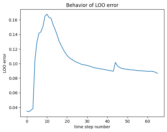
Despite the large number of samples, I still get large errors (maximum LOO error \approx 0.17) which is too much for reliable Sobol indices computation (I have read in another post that it should be around 10^{-2}).
Do you have an idea on how I could reduce the PCE LOO error in order to make it suitable for reliable Sobol indices computation ?
Thank you in advance for your precious help.
Below is the code I am using to build the PCE, if you want to have a look.
Best regards,
Guillaume
The samples files are too large for me to upload here, but here is the code I am using to build the PCE :
#STEP2 : Retrieve simulation data
simfiles_dir = 'Res_10ksim/'

# first set of simulation results
Y_E2_1 = np.loadtxt(simfiles_dir+'GSA31_E2.csv', delimiter = ',')

X1 = np.loadtxt(simfiles_dir+'GSA31_X.csv', delimiter = ',')


# second set of simulation results
Y_E2_2 = np.loadtxt(simfiles_dir+'GSA32_E2.csv', delimiter = ',')

X2 = np.loadtxt(simfiles_dir+'GSA32_X.csv', delimiter = ',')


Y_E2_3 = np.loadtxt(simfiles_dir+'GSA33_E2.csv', delimiter = ',')

X3 = np.loadtxt(simfiles_dir+'GSA33_X.csv', delimiter = ',')


Y_E2_4 = np.loadtxt(simfiles_dir+'GSA34_E2.csv', delimiter = ',')

X4 = np.loadtxt(simfiles_dir+'GSA34_X.csv', delimiter = ',')


X = np.concatenate((X1,X2,X3,X4))
Y_E2 = np.concatenate((Y_E2_1,Y_E2_2,Y_E2_3,Y_E2_4))

nanidx = np.argwhere(np.isnan(Y_E2[:,0]))

Y_E2 = np.delete(Y_E2, nanidx, 0)
X = np.delete(X, nanidx, 0)

#split into calibration/validation set (here, size : 0.75 / 0.25)

Ncal = int(3*(int(X.shape[0]/4)))

X_cal = X[:Ncal]
Y_E2_cal = Y_E2[:Ncal]


X_val = X[Ncal:]
Y_E2_val = Y_E2[Ncal:]

print(X_cal.shape)
print(Y_E2_cal.shape)

print(X_val.shape)
print(Y_E2_val.shape)
Output :
(7482, 22)
(7482, 66)
(2495, 22)
(2495, 66)
# STEP 3 : probabilistic model input

InputOpts = {
    "Marginals": [
        # Layer 1
        {"Type": "Uniform",
         "Parameters": [0, 3] # log10Ks1
        },
        {"Type": "Uniform",
         "Parameters": [0.01, 0.04] # tr1
        },
        {"Type": "Uniform",
         "Parameters": [0.30, 0.50] #ts1
        },
        {"Type": "Uniform",
         "Parameters": [0.01, 0.15] # alpha1
        },
        {"Type": "Uniform",
         "Parameters": [1, 1.8] # n1
        },
        # Layer 2
        {"Type": "Uniform",
         "Parameters": [0, 3] # log10Ks2
        },
        {"Type": "Uniform",
         "Parameters": [0.01, 0.04] # tr2
        },
        {"Type": "Uniform",
         "Parameters": [0.30, 0.50] #ts2
        },
        {"Type": "Uniform",
         "Parameters": [0.01, 0.15] # alpha2
        },
        {"Type": "Uniform",
         "Parameters": [1, 1.8] # n2
        },
        # Layer 3
        {"Type": "Uniform",
         "Parameters": [0, 3] # log10Ks3
        },
        {"Type": "Uniform",
         "Parameters": [0.01, 0.04] # tr3
        },
        {"Type": "Uniform",
         "Parameters": [0.30, 0.50] #ts3
        },
        {"Type": "Uniform",
         "Parameters": [0.01, 0.15] # alpha3
        },
        {"Type": "Uniform",
         "Parameters": [1, 1.8] # n3
        },
        # Non simulated zone parameters
        {"Type": "Uniform",
         "Parameters": [0.01, 0.05] # tRMP1
        },
        {"Type": "Uniform",
         "Parameters": [0, 1e-8] # tRMP2
        },
        {"Type": "Uniform",
         "Parameters": [0, 1e-8] # tRMP3
        },
        # Field capacity parameter
        {"Type": "Uniform",
         "Parameters": [0.20, 0.30] # theta_c1
        },
        {"Type": "Uniform",
         "Parameters": [0.20, 0.30] # theta_c2
        },
        {"Type": "Uniform",
         "Parameters": [0.20, 0.30] # theta_c3
        },
        # delta_h piezo
        {"Type": "Uniform",
         "Parameters": [-20.0, 20.0]
        },
    ]
}

myInput = uq.createInput(InputOpts)

MetaOpts = {
    'Type': 'Metamodel',
    'MetaType': 'PCE'
}

# Use experimental design loaded from the data files:


MetaOpts['ExpDesign'] = {
    'X': X_cal.tolist(),
    'Y': Y_E2_cal.tolist()
}

#Set the maximum polynomial degree to 5:

MetaOpts["Degree"] = np.arange(1,5).tolist()

# Specify the parameters of the PCE truncation scheme

MetaOpts['TruncOptions'] = {
    'qNorm': 0.7,
    'MaxInteraction': 2
}


#Provide the validation data set to get the validation error:

MetaOpts['ValidationSet'] = {
    'X': X_val.tolist(),
    'Y': Y_E2_val.tolist()
}

# Create the PCE metamodel:

myPCE_E2 = uq.createModel(MetaOpts)

# Print a summary of the resulting PCE metamodel:
uq.print(myPCE_E2)
Output :
Warning: The selected PCE has more than 1 output. Only the 1st output will be
printed
In uq_PCE_print (line 12)
In uq_print_uq_metamodel (line 16)
In uq_module/Print (line 52)
In uq_print (line 29)
In uq_web_cli_filebased (line 301)
You can specify the outputs you want to be displayed with the syntax:
uq_display(PCEModule, OUTARRAY)
where OUTARRAY is the index of desired outputs, e.g. 1:3 for the first three
------------ Polynomial chaos output ------------
Number of input variables: 22
Maximal degree: 4
q-norm: 0.70
Size of full basis: 782
Size of sparse basis: 141
Full model evaluations: 7482
Leave-one-out error: 3.4710601e-02
Modified leave-one-out error: 3.6061287e-02
Validation error: 3.6288626e-02
Mean value: 72.7910
Standard deviation: 43.7980
Coef. of variation: 60.169%
--------------------------------------------------
Retrieving maximum LOO error on the trained PCE :
LOO_errors_2 = []
for i in range(len(myPCE_E2['Error'])):
    LOO_errors_2.append(myPCE_E2['Error'][i]['LOO'])

max(LOO_errors_2)
Output : 0.16775668945295738