Ishigami Function
The Ishigami function is commonly used as a test function to benchmark global sensitivity analysis methods (Ishigami and Homma, 1990; Sobol’ and Levitan, 1999; Marrel et al., 2009).
Description
The analytic expression of the Ishigami function is given as:
where \mathbf{x} = \{x_1, x_2,x_3\} \in [-\pi, \pi]^3 are input variables; while a and b are parameters.
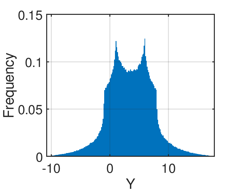
Figure 1: The histogram of the Ishigami function based on 10^6 sample points.
Inputs
For computer experiment purposes, the inputs x_1, x_2, x_3 are modeled as three independent uniform random variables.
| No | Variable | Distribution | Parameters |
|---|---|---|---|
| 1 | x_1 | Uniform |
x_{1,\min} = -\pi, x_{1,\max} = \pi |
| 2 | x_2 | Uniform |
x_{2,\min} = -\pi, x_{2,\max} = \pi |
| 3 | x_3 | Uniform |
x_{3,\min} = -\pi, x_{3,\max} = \pi |
Parameters
The parameters of the Ishigami function differ according to the literature as shown in the table below.
| No | Value | Source |
|---|---|---|
| 1 |
a = 7 b = 0.1 |
Marrel et al. (2009) |
| 2 |
a = 7 b = 0.05 |
Sobol’ and Levitan (1999) |
Reference values
First-order Sobol’ indices
The analytical solution for the first-order Sobol’ indices of the Ishigami function as described above is:
- S_1 = \frac{V_1}{\mathbb{V}[Y]}
- S_2 = \frac{V_2}{\mathbb{V}[Y]}
- S_3 = \frac{V_3}{\mathbb{V}[Y]} = 0
where:
- \mathbb{V}[Y] = \frac{a^2}{8} + \frac{b\pi^4}{5} + \frac{b^2\pi^8}{18} + \frac{1}{2}
- V_1 = 0.5 (1 + \frac{b\pi^4}{5})^2
- V_2 = \frac{a^2}{8}
- V_3 = 0
Total-effect Sobol’ indices
The analytical solution for the total-effect Sobol’ indices of the Ishigami function as described above is:
- S_{T1} = \frac{V_{T1}}{\mathbb{V}[Y]}
- S_{T2} = \frac{V_{T2}}{\mathbb{V}[Y]}
- S_{T3} = \frac{V_{T3}}{\mathbb{V}[Y]}
where:
- V_{T1} = 0.5 (1 + \frac{b\pi^4}{5})^2 + \frac{8b^2\pi^8}{225}
- V_{T2}= \frac{a^2}{8}
- V_{T3} = \frac{8b^2\pi^8}{225}
Resources
The vectorized implementation of the Ishigami function in MATLAB as well as the script file with the model and probabilistic inputs definitions for the function in UQLAB can be downloaded below:
uq_ishigami.zip (2.2 KB)
The contents of the file are:
| Filename | Description |
|---|---|
uq_ishigami.m |
vectorized implementation of the Ishigami function in MATLAB |
uq_Example_ishigami.m |
definitions for the model and probabilistic inputs in UQLab |
LICENSE |
license for the function (BSD 3-Clause) |
References
- T. Ishigami and T. Homma, “An importance quantification technique in uncertainty analysis for computer models,” In the First International Symposium on Uncertainty Modeling and Analysis, Maryland, USA, Dec. 3–5, 1990. DOI:10.1109/SUMA.1990.151285
- I. M. Sobol’ and Y. L. Levitan, “On the use of variance reducing multipliers in Monte Carlo computations of a global sensitivity index,” Computer Physics Communications, vol. 117, no. 1, pp. 52–61, 1999. DOI:10.1016/S0010-4655(98)00156-8
- A. Marrel, B. Iooss, B. Laurent, and O. Roustant, “Calculations of Sobol indices for the Gaussian process metamodel,” Reliability Engineering & System Safety, vol. 94, no. 3, pp. 742–751, 2009. DOI:10.1016/j.ress.2008.07.008
