I read Data-driven polynomial chaos expansion for machine learning regression. According to the paper, a good result can be obtained by declaring a polynomial type arbitrary when it is difficult to determine the dependency of an input variable.
In uq_Example_PCE_06_ArbitraryBasis of uqlab example, input variable is declared as gaussian and polytype uses Legendre. But isn’t it right to use Hermite when the input distribution is gaussian?
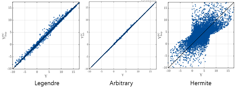
Results of polytype changes for three gaussian inputs. Legendre, Hermite, Arbitrary (from left to right)
In addition, if the input forms a known distribution such as perfect gaussian or beta, it is easy to determine the parameters of the distribution. However, if the distribution of inputs is not clear, are they often assume to uniform?
Thanks for your interesting question. There are actually two questions
Regarding uq_Example_PCE_06_ArbitraryBasis
This examples assumes truncated Gaussian distributions as inputs. As you can see by typing uq_display(myInput), due to truncation this input distribution is far from a Gaussian one.
The first part of the example forces UQLab to use Legendre polynomials. To do this, internally an isoprobabilistic transform \mathbf{X} = \mathcal{T}(\mathbf{U}) is used, where \mathbf{U} = (U_1, U_2, U_3) are uniform variables over [-1,1]. What is represented as a PCE is not the function Ishigami(\mathbf{X}), but the composed function Ishigami(\mathcal{T}(\mathbf{U})). As the shape of the (truncated) input is not too far from a uniform distribution, this transform \mathcal{T} is fairly linear, and the (Legendre) PC expansion results are fairly good.
In the second part of the script, arbitrary PCE is used, where the orthogonal polynomials are computed w.r.t. the true truncated Gaussian inputs, meaning that there is no transform \mathcal{T}. Obviously the results are better.
In your post, you tried a third option (not present in the original UQLab example), where you force UQLab to use Hermite polynomials. What happens now is that a transform \mathcal{T}_2 is used, from truncated Gaussian (the input) to standard normal variables (\mathbf{\xi}_1, \mathbf{\xi}_2, \mathbf{\xi}_3)\!. As this truncation is highly non linear due to the unbounded support of the standard normal variables, the function Ishigami(\mathcal{T}_2(\mathbf{\xi})) is much more difficult to approximate with a Hermite PCE, thus the bad results you get.
As a conclusion, when you have fancy input distributions, use arbitrary PCE ! NB: this is the default in UQLab if you don’t specify anything.
Regarding dependence in the input raw data
What you show in the paper you mention (available here as a preprint), is that when you have raw data (and no input distributions) as it is usual in machine learning settings, you can use PCE to build a model.
The first option would be to build a detailed statistical model of the input data, using copulas when there is statistical dependence between inputs. Then an isoprobabilistic transform must be used before building a PCE (which can be non linear, as the Example_6 above)
The second option is to simply ignore that there is dependence to build the PCE. In this case, you use kernel smoothing densities for each parameter separately, and arbitrary PCE w.r.t this densities.
In terms of quality of the resulting model (as measured from the error on a validation set), the second option reveals much better, again between you don’t include the very non linear transform in the game, … and it is also easier to implement since you don’t need at all to infer the dependence (copula) model between your inputs.
I hope this answers your question.
Best regards
Bruno