Hi everyone.
I would like to ask question about PCE and also the sensitivity analysis. I have 800 output results based on 800 LHS samples with 7 random variables, running in FEM software. Based on the example “PCE from existing data”, the PCE metamodel was built and had a pretty good validation.
Below is my input data:
%% 4 - PROBABILISTIC INPUT MODEL
InputOpts.Marginals(1).Name = ‘DcRef’;
InputOpts.Marginals(1).Type = ‘Lognormal’;
InputOpts.Marginals(1).Moments = [3e-11 0.6e-11];
InputOpts.Marginals(2).Name = ‘mc’;
InputOpts.Marginals(2).Type = ‘Beta’;
InputOpts.Marginals(2).Parameters = [9.2944 52.6685 0 1];
InputOpts.Marginals(3).Name = ‘Uc’;
InputOpts.Marginals(3).Type = ‘Beta’;
InputOpts.Marginals(3).Parameters = [0.4437 0.1268 32e3 44.6e3];
InputOpts.Marginals(4).Name = ‘depth’;
InputOpts.Marginals(4).Type = ‘Gaussian’;
InputOpts.Marginals(4).Parameters = [0.04 0.01];
InputOpts.Marginals(4).Bounds = [0.01 inf];
InputOpts.Marginals(5).Name = ‘Xr’;
InputOpts.Marginals(5).Type = ‘Gaussian’;
InputOpts.Marginals(5).Parameters = [0.01 0.001];
InputOpts.Marginals(5).Bounds = [0 inf];
InputOpts.Marginals(6).Name = ‘Cfevn’;
InputOpts.Marginals(6).Type = ‘Lognormal’;
InputOpts.Marginals(6).Moments = [7.35 5.145];
InputOpts.Marginals(7).Name = ‘Cth’;
InputOpts.Marginals(7).Type = ‘Gaussian’;
InputOpts.Marginals(7).Parameters = [2 0.4];
% Create an INPUT object based on the specified marginals:
myInput = uq_createInput(InputOpts);
%% 4 - POLYNOMIAL CHAOS EXPANSION (PCE) METAMODEL
% Select PCE as the metamodeling tool:
MetaOpts.Type = ‘Metamodel’;
MetaOpts.MetaType = ‘PCE’;
MetaOpts.Input = myInput;
%%
% Use experimental design loaded from the data files:
MetaOpts.ExpDesign.X = X;
MetaOpts.ExpDesign.Y = Y;
%%
% Set the maximum polynomial degree to 5:
MetaOpts.Degree = 1:5;
%%
% Provide the validation data set to get the validation error:
MetaOpts.ValidationSet.X = Xval;
MetaOpts.ValidationSet.Y = Yval;
%%
% Create the metamodel object and add it to UQLab:
myPCE = uq_createModel(MetaOpts);
%%
% Print a summary of the resulting PCE metamodel:
uq_print(myPCE)
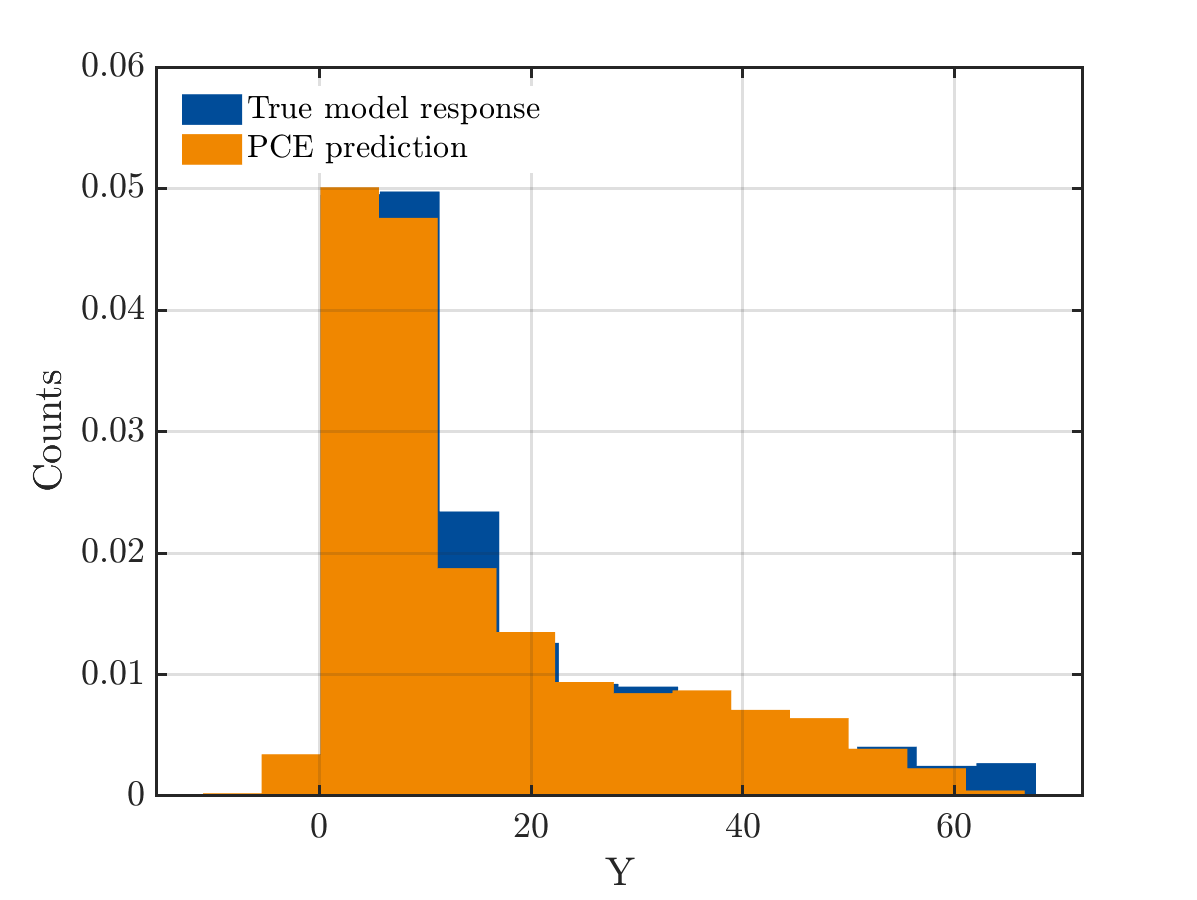
Below is the comparision of True model response and PCE model
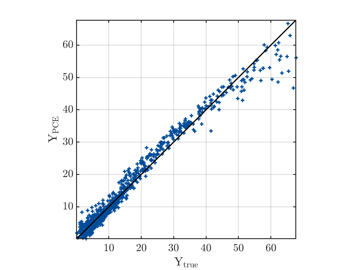
And the true output and PCE output
The result from UQlab is shown below:
−−−−−−−−−−−−Polynomialchaosoutput−−−−−−−−−−−−
Number of input variables: 7
Maximal degree: 3
q-norm: 1.00
Size of full basis: 120
Size of sparse basis: 64
Full model evaluations: 788
Leave-one-out error: 3.3906646e-02
Modified leave-one-out error: 4.5942902e-02
Validation error: 2.6473454e-02
Mean value: 34.6734
Standard deviation: 49.1539
Coef. of variation: 141.762%
−−−−−−−−−−−−−−−−−−−−−−−−−−−−−−−−−−−−−−−−−−−−−−−−−−
PCE metamodel validation error: 2.6473e-02
PCE metamodel LOO error: 3.3907e-02
The mean value from UQlab is far from the mean value of real data, and as I read in some discussion available in UQlab forum, it does not mean I got the wrong PCE, but it is an arbitrary PCE. Therefore, the mean and the standard deviation of aPCE does not express the real mean and Std of the model. I have checked manually by comparing mean(YPCE) and mean(Yval) and they are the same, so I think the model is still right. My questions are:
- Is there any way to transfer from arbitrary PCE to orthogonal PCE?
- If not, can I do the Sobol’s sensitivity analysis on arbitrary PCE?
- If I have the results of 800 simulations, can I use 800 samples for experimental design and also use the same 800 outputs for validation set?
I really appreciate any support and response from you.
Thank you so much.