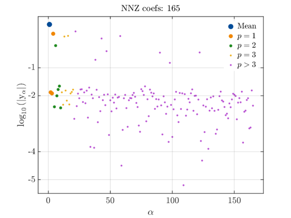
the attached figure plots the magnitude of the PCE coefficients as a function of their enumeration, i.e. the a_j's in the equation Y = \displaystyle{\sum_{j=0}^{P-1} a_j \, \Psi_j(\textbf{X})} as a function of j. As the basis of \Psi_j(\textbf{X})'s is orthonormal, it is licit to compare the magnitude of the coefficients.
Moreover, the coefficients of the low-degree polynomials are to the left in this figure: the mean value is a_0 as you can see. What we see in this figure, where the y-axis is in log scale, is that most coefficients have a magnitude 2 to 3 orders smaller than the largest coefficients. Remember that the variance of the response \textrm{Var}\left[ \textbf{X}\right] = \displaystyle{\sum_{j=1}^{P-1} a_j^2}: a coefficient that is 3 orders of magnitude smaller than a_0 contributes to 10^{-6} to this variance, i.e., is completely negligible. This is because of this strong decay in the coefficients magnitude that PC expansions converge rather fast.
The figure also shows that we cannot truncate the series by the largest polynomial degree: we see with the purple points that several non negligible coefficients (> 0.1 a_0) correspond to \Psi_j's of degree larger than 3: we need sparse polynomial chaos expansions to address this efficiently, that is, a sparse solver which directly finds and computes only the coefficients with largest magnitude, see e.g. Blatman & Sudret (2011); Lüthen et al (2021).
Best regards
Bruno
References
Blatman, G., Sudret, B., 2011. Adaptive sparse polynomial chaos expansion based on Least Angle Regression. Journal of Computational Physics 230, 2345–2367. https://doi.org/10.1016/j.jcp2010.12.021
Lüthen, N., Marelli, S., Sudret, B., 2021. Sparse polynomial chaos expansions: Literature survey and benchmark. SIAM/ASA Journal on Uncertainty Quantification 9, 593–649. https://doi.org/10.1137/20M1315774