Introduction
A key step in an uncertainty quantification (UQ) study is to define the distributions that will be used to represent the uncertainty in the input parameters of a computational model of interest. Referring to the global framework for UQ that is discussed here, this step is called Quantification of the sources of uncertainty (Step B).
Probabilistic input for model exploration
As soon as a computational model has been developed, one is often interested in investigating what happens when we change some parameters from their nominal (“best estimate”) values to other smaller or larger values. This type of analysis is known as model exploration. In this context, we usually assign to each parameter a reasonable lower bound x_l and upper bound x_u based on expert knowledge on the model, literature data, etc.
When only the bounds are known and no additional information on more/less likely values is available, the suitable distribution for the parameter is a uniform distribution over the interval defined by the two bounds:
This distribution satisfies the principle of maximum entropy when only bounds are known.
Remark
Model exploration can be carried out by computing the Sobol’ global sensitivity indices of the model response, which characterize the contribution of each input parameter (or combination of parameters) to the output variance. This allows for identifying important parameters (i.e. the ones whose variation influence the model output) from the unimportant parameters (i.e the ones that do not influence the output, and thus could simply be fixed to a single value without changing the nature of the analysis). Sobol’ indices can also provide valuable information about the interactions between the input parameters.
Probabilistic input for aleatory uncertainty (No data available)
In certain applications, it is not possible to assign a single value to a parameter because this parameter is known to naturally vary. This is typically the case for parameters describing material properties in engineering applications (e.g. material elastic behavior, strength, toughness, thermal conductivity, electromagnetic permittivity, etc.) or environmental conditions (e.g. temperature, climatic loads, etc.).
In such situations, it is important to select distributions that are consistent with physical constraints, such as positivity, boundedness, special behavior in extreme values (tail dependence), etc. As an example:
- Material properties that are positive in nature are usually well-represented by lognormal distributions. Gaussian distributions should be avoided, especially in cases where the coefficient of variation[1] is large, which would give frequent negative non-physical realizations and troubles in the uncertainty propagation phase. Truncated Gaussian may be used, however it may lead to unrealistic shapes of the resulting distribution.
- Gaussian distributions are often used for modelling the uncertainties of elements’ dimensions (lengths) in engineering systems. This allows one to represent the scattering of the real dimensions of the system during the manufacturing process because of tolerances. In this case, the coefficient of variation is usually so low that there is no issue with positiveness.
- If a parameter is bounded in nature (e.g. the Poisson’s ratio in elasticity), a bounded distribution such as the beta distribution is to be used instead.
- If a parameter represents some maximum value over a time period (e.g. climatic loads, the water level in a river, etc.), it can be modeled with one of the so-called extreme value distributions such as Gumbel or Weibull.
Remark
It is important to realize that selecting a suitable distribution based on the current level of knowledge is always possible, even if there is no measured data available.
Probabilistic input for aleatory uncertainty (Sufficient data available)
In cases where there is evidence of the natural variability of a parameter because of observed scattered values \mathcal{X} = \{x_1, \, \cdots, x_n\}, statistical inference can be used to build a probabilistic model, as soon as reasonable number of points is available (typically, n \ge 30).
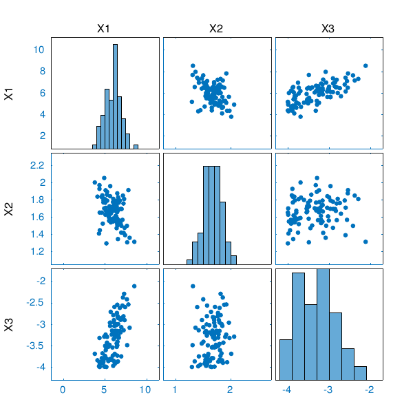
- Numerical summaries and graphics are used to represent the data, i.e. empirical CDFs (cumulative distribution functions), histograms, “kernel smoothing” densities, etc. Scatterplots can be used to plot the correlation between pairs of parameters.
- Based on visual inspection, assumptions are made on the distribution families that could fit the data. This means selecting a parametric family such as Gaussian, lognormal, Gamma, Beta, etc.
- Under the assumption that parameter X follows a distribution f_{X} parametrized by a vector of hyperparameters \boldsymbol{\theta}:
the goal of statistical inference is to find the best estimator \hat{\boldsymbol{\theta}} so that f_X fits the data in \mathcal{X}. The most common methods to fit the parameters are:
- the method of moments, in which the empirical moments of the sample \mathcal{X} are set equal to the moments of the distribution f_X, and the resulting equations solved for \hat{\boldsymbol{\theta}};
- maximum likelihood estimation, in which the likelihood of the sample set is maximized as a function of \boldsymbol{\theta}.
When several candidate distributions are fitted, they can be compared using a model selection criterion such as the Akaike information criterion (AIC) or the Bayesian information criterion (BIC).
What to do in case of limited data?
There are practical situations in which data is scarce, i.e. where only a handful of data points is available, which does not allow us to use standard statistical inference. In this case, Bayesian statistics may be used to combine prior knowledge on the distribution of X and its hyperparameters together with the scarce data. Prior knowledge can be represented by following the same procedure as for the case of no data available, i.e. by applying the maximum entropy principle to the available knowledge of the problem.
In the Bayesian paradigm, the hyperparameters \boldsymbol{\theta} themselves are treated as random variables, which are given a distribution that reflects the prior knowledge. For instance:
X follows a Gaussian distribution with mean value \mu, which belongs to a given range [m_l, \, m_u]:
X \sim \mathcal{N}(x;\; \mu, \sigma^2) \quad \textsf{where} \quad \mu \sim\mathcal{U}(\mu; [m_l, \, m_u])
The data gathered in \mathcal{X} allows one to update the distribution of \mu and get a posterior distribution, which can then be used to define the distribution of X.
Conclusions
Whatever the available amount of information and data, it can be used to build a probabilistic model for further uncertainty propagation. The construction of such a probabilistic model should not be overlooked: the subsequent results in terms of output distribution, important parameters or probability of threshold exceed will depend on this choice. The “good practices” summarized above can be used as a starting point. In any case, uninformed choices such as “I use a Gaussian distribution with 10% coefficient of variation for all parameters”, which is often seen in practice, should be absolutely avoided.
Back to the Chair’s Blog index
Notes
The coefficient of variation of a random variable is defined as the ratio of its standard deviation to its mean value (when the latter is non zero). ↩︎