The high-dimensional limit state function is used to test algorithms in structural reliability analysis, such as Adaptive Kriging Monte Carlo simulation (AK-MCS) and others (Rackwitz, 2001). A prominent feature of this test function is that the failure probability does not change significantly when changing the number of input dimensions.
Description
The analytic expression of the high-dimensional limit state function is given as:
where M is the number of input variables (or dimensions; positive integer); \{x_m\}_{m=1}^{M} are the input variables; and a is a parameter. By default, the parameter is set to 0.2.
The failure event is defined as g(\mathbf{x}) \leq 0 and the failure probability P_f = \mathbb{P}[g(\mathbf{x}) \leq 0]. Figure 1 and 2 show the surface and contour plots of the 2-dimensional high-dimensional function using the default values of the constants, respectively.
In Figure 2, the limit state function at which g(\mathbf{x}) = 0 is highlighted.
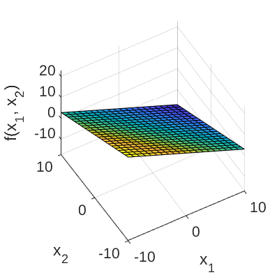
Figure 1: Surface plot of the 2-dimensional high-dimensional limit state function.
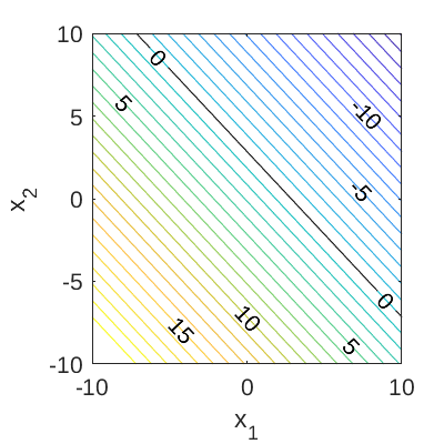
Figure 2: Contour plot of the 2-dimensional high-dimensional limit state function. The limit state function at which g(\mathbf{x})=0 is also shown.
Inputs
M independent identically distributed lognormal random variables are considered for the high-dimensional limit state function.
| No | Variable | Distribution | Parameters |
|---|---|---|---|
| 1 | x_1 | Lognormal |
\mu_{x_1} = 1, \sigma_{x_1} = 0.2 |
| \vdots | \vdots | \vdots | \vdots |
| M | x_M | Lognormal |
\mu_{x_M} = 1, \sigma_{x_M} = 0.2 |
Parameter
By default, the parameter a is set to 0.2 following Rackwitz (2001).
Reference values
The asymptotic value of the failure probability P_f with M \rightarrow \infty is 1.35 \times 10^{-3} (Rackwitz, 2001). Some other values of P_f calculated using different methods for different values of M are shown in the table below.
| Method | M | N | \hat{P}_f | \text{CoV}[\hat{P}_f] | Source |
|---|---|---|---|---|---|
| FORM | 50 | 154 | 1.531 \times 10^{-4} | - | Rackwitz (2001) |
| SORM | 50 | 1'480 | 2.555 \times 10^{-3} | - | Rackwitz (2001) |
| MCS | 50 | 10^{6} | 1.915 \times 10^{-3} | 2.28\% | UQLab v1.2.1 |
| FORM | 100 | 304 | 3.369 \times 10^{-4} | - | Rackwitz (2001) |
| SORM | 100 | 5'455 | 2.98 \times 10^{-3} | - | Rackwitz (2001) |
| MCS | 100 | 10^{6} | 1.685 \times 10^{-3} | 2.43\% | UQLab v1.2.1 |
| FORM | 100 | 603 | 6.212 \times 10^{-6} | - | Rackwitz (2001) |
| SORM | 200 | 20'904 | 4.53 \times 10^{-3} | - | Rackwitz (2001) |
| MCS | 200 | 10^{6} | 1.669 \times 10^{-3} | 2.45\% | UQLab v1.2.1 |
Resources
The vectorized implementation of the high-dimensional limit state function in MATLAB as well as the script file with the model and probabilistic inputs definitions for the function in UQLAB can be downloaded below:
uq_highDimensional.zip (2.4 KB)
The contents of the file are:
| Filename | Description |
|---|---|
uq_highDimensional.m |
vectorized implementation of the high-dimensional limit state function in MATLAB |
uq_Example_highDimensional.m |
definitions for the model and probabilistic inputs in UQLab |
LICENSE |
license for the function (BSD 3-Clause) |
Reference
- R. Rackwitz, “Reliability analysis—a review and some perspectives,” Structural Safety, vol. 23, no. 4, pp. 365–395, 2001. DOI:10.1016/S0167-4730(02)00009-7