Hi @paulremo, (Hello also to anyone else who is interested in this topic)
Thanks for your support and for your suggestions.
I like the idea of using a name-value pair as parameters for uq_display_uq_inversion to allow
some changes in the plots without requiring further calls of uq_postProcessInversion, but
there are some issues one needs to decide/consider before it can be implemented:
-
Are your examples supposed to be
a) options related only to the plots activated/deactivated in the current UQLab implementation by the ‘‘predDist’’ flag, and maybe the new plots suggested in my post, or
b) option for all plot types generated byuq_display_uq_inversion?
The answer a) fits to the name of the option and the name of the name for the local variable in your example, but in addition tomyPredDistOpts.Sample.PostPredthere is also a flag
myPredDistOpts.Sample.Post, seeming to be a switch for activating/deactivating the generation of the scatter plot for the posterior density, Hence, it seems to me that you may had somehow the situation b) in mind when writing your example, at least subconsciously.
But, if you really want to use the ansatz in b), I suggest to change the name for the name-value pair, and of the variable in the discussion, e.g. replacing'PredDist'by the a new name, like e.g.'plotOpts'or'dispOpts'. Moreover, I would suggest to denote flags for scatter plots byScatter. Hence,myPredDistOpts.Sample.Postmay be replaced bymyPlotOpts.Scatter.Post.
But, i must admit that I do not know, what could be good common start for the options related to the plots generated bymod_UQLab_plotSeriesPred_2021.mand andplotSeriesPred.mi.e.
for'PostPred','PriorPred','Model'or'ModelAtPost','Model(PE)+noise', or
'Model(PE)+noise:edges'(see below).
(Side remark: I have now performed many Bayesian Inversions using UQLab without being interested in the prior scatter plot. Here, it became my habit to simply ignore the
created scatter plot for the prior, and I think that in general I would be to lazy to stop the
creation of this plot by using some flag/parameter in the code. But maybe other users would like
to use this flag, and even I may like to use it if I perform that many Bayesion inversion in one program run such that the number of created windows may become to large, i.e. larger then 100–120, and could maybe force a freze of matlab or of my whole laptop. ) -
It is my interpretation of your example that you suggest to use flags to activate/deactivate the possible plots components in a new version of
plotSeriesPred.mthat is using parts ofmod_UQLab_plotSeriesPred_2021.m. If this interpretation is correct, one has to think on the order of the creating of the plots, such that hiding of interesting parts is reduced:
I think that a good order of plots would be
1.'PriorPred': plot of prior predictive density, i.e. (model output at priori samples) + noise,
2.'PostPred': plot of posterior predictive density, i.e. ( model output at posterior samples) + noise,
3.'Model(PE)+noise': plot of (model output at point estimate) + noise,
4. ’Model'or' ModelAtPost': plot of model output at posterior samples ,
5.'Model(PE)+noise:edges': plot of boundary of violin plot for (model output at point estimate) + noise region, now shown with an connected line.
(This is supposed to be typically combined with the'PostPred'Plot, such that one can compare the result of (full) forward UQ and simplified forward UQ.
-
If
myPredDistOpts.Range = [1:10, 200:210];indicates to replace myStartIndandEndIndinput values leading to the plot rangeStartInd,…,EndIndby a more general set of numbers as plot range, one has to change some parts of the code inmod_UQLab_plotSeriesPred_2021.mthat make use on the current form of the plot range.
Moreover, one should spend some time on considering to update the generation of tic and of the tic numbers at the x axis, if one is allowing general points sets, like, e.g.[1,3,6,9:11,16,19,20,23,25,42,45,47,48,50,51,70,71,73,79,80,81,84,88,90,93,94]. Currently, maximal 10 numbers are shown, but by counting one can figure out for each ``violin plot’’ the corresponding index. How to deal with a more general situation requires some further consideration.Therefore, I think that one has to decide if using the general plot range instead of
StartInd,…,EndIndis worth the induced further work and complexity. -
Moreover, for the plot range one also needs to take into account that there can be multiple data groups such that one needs to define the plat range for each of these groups. To formulate this in way that is correct UQLab style need as least some considerations.
-
In addition, one may have to decide if also a scalar version of the plots 3) – 5) in point 2 is needed, or if is is sufficient to provide the possibility to create of the violin plots also in the case of a scalar model output.
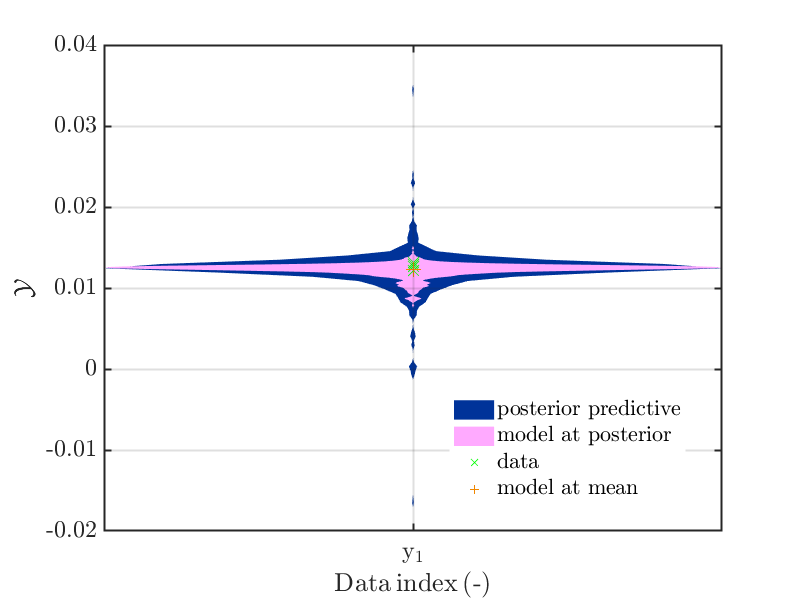
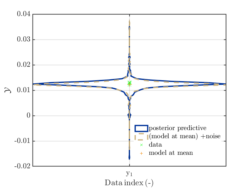
Examples of the corresponding plots can be generate with my current function
byuq_Example_Inversion_01_Beam myData = myBayesianAnalysis.Data mySamples.PostPred= myBayesianAnalysis.Results.PostProc.PostPredSample.PostPred mySamples.Post= myBayesianAnalysis.Results.PostProc.PostPredSample.Post myPointEstimate=myBayesianAnalysis.Results.PostProc.PointEstimate.ForwardRun mod_UQLab_plotSeriesPred_2021(mySamples,myData,'post&Model',myPointEstimate) mod_UQLab_plotSeriesPred_2021(mySamples,myData, ... 'post&Model(PE)+noise:edges', myPointEstimate)
leading to the plots


-
Moreover, a further possible parameter may be a field
xPosof the length of the data vector such thatxPos(i)provides the horizontal position to be used for the center of violin plot for the data pointi.
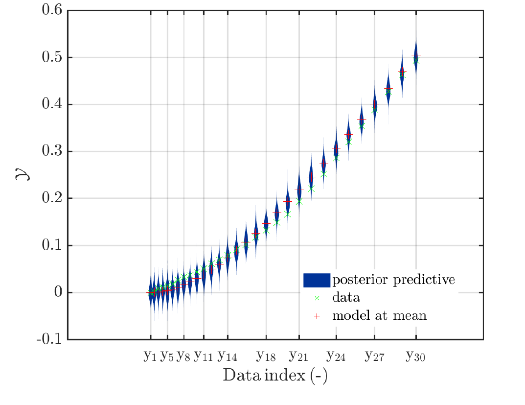
This could be (a linear transformattion of) the values for some non-UQ input parameter that is evaluated in the model, like e.g. q_i in the Topic: Bayesian inversion for structural parameter identification (the load varies in each measurement ) or the load values in the Topic: Bayesian inference with changing (known) model parameters.The generated plots should allow to get some impression of the dependence of the derived results on this non-UQ input parameter. This may require some considerations how to scale the size violin plots in the code, or some considerations/ try and error cyclus for the UQLab-User how to transform to values the non-UQ input parameter to get a plot with violin plots in an appropriate size.
I created modifications of ‘‘plotSeriesPred.m’’ that are generating this kind of plots, an example is shown below. Since this modification is also an example of dirty coding style, I do not dare to provide it here in its current form.

Scr_extr_UQLab_3rd_combi_reload-fig28.png
- I created serveral modefications
plotSeriesPred.msuch that I could use them to
combine serveral plots into one plot, using the provided likexPosin point 6 combined with
plot of a subrange using that this function only deal with one plot in one call. To allow this kind of combination in a way that is an appropriate UQLab way may require some work and I do not
know if anyone else may need this possibility.
Okay, I think this post is already quite long and should provide some possibilities for discussion.
Greetings
Olaf