The 2-dimensional four-branch function is a common benchmark problem in reliability analysis (Schueremans and van Gemert, 2005; Echard et al., 2011; Schöbi et al., 2017). The function describes the failure of a series system with four distinct limit state components.
Description
The mathematical formulation of the four-branch function reads:
where the input variables \mathbf{x} = \{x_1, x_2\} are modeled as two independent Gaussian random variables and p is a constant parameter. The default constant parameter value is 6.
The failure event is defined as f(\mathbf{x}) \leq 0 and the failure probability P_f = \mathbb{P}[f(\mathbf{x}) \leq 0]. Figure 1 and 2 show the surface and contour plot of the four-branch function, respectively. In Figure 2, the limit state function (f(\mathbf{x}) = 0) is shown.
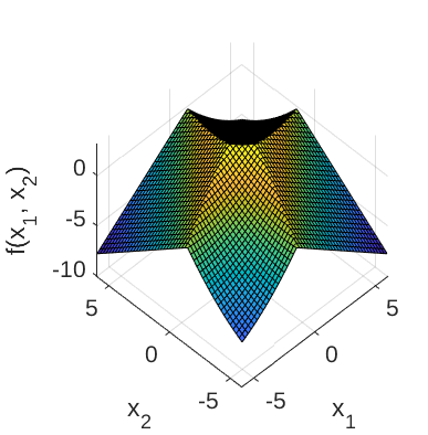
Figure 1: Surface plot of the four-branch function.
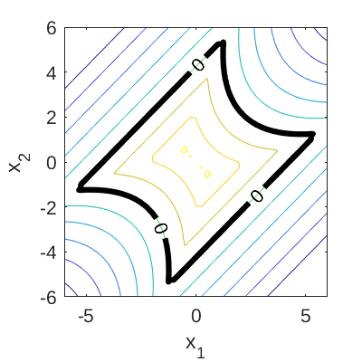
Figure 2: Contour plot of the four-branch function. The limit state function is also shown.
Inputs
The two input variables are modeled as independent Gaussian random variables.
| No | Variable | Distribution | Parameters |
|---|---|---|---|
| 1 | x_1 | Gaussian |
\mu_{x_1} = 0 \sigma_{x_1} = 1 |
| 2 | x_2 | Gaussian |
\mu_{x_2} = 0 \sigma_{x_2} = 1 |
Constant parameter
The default value of the constant parameter p is 6.
Reference values
Some reference values for the failure probability P_f from the literature are shown in the table below.
| Method | N | \hat{P}_f | \text{COV}[\hat{P}_f] | Source |
|---|---|---|---|---|
| MCS | 10^8 | 4.460 \times 10^{-3} | 1.5\% | Schöbi et al. (2017) |
| MCS | 10^6 | 4.416 \times 10^{-3} | 0.15\% | Echard et al. (2011) |
| IS | 1469 | 4.9 \times 10^{-3} | - | Echard et al. (2011) |
Resources
The vectorized implementation of the four-branch function in MATLAB as well as the script file with the model and probabilistic inputs definitions for the function in UQLAB can be downloaded below:
uq_fourBranch.zip (2.5 KB)
The contents of the file are:
| Filename | Description |
|---|---|
uq_fourBranch.m |
vectorized implementation of the four-branch function |
uq_Example_fourBranch.m |
definitions for the model and probabilistic inputs in UQLab |
LICENSE |
license for the function (BSD 3-Clause) |
References
- B. Echard, N. Gayton, and M. Lemaire, “AK-MCS: An active learning reliability method combining Kriging and Monte Carlo simulation”, Reliability Engineering and System Safety, vol. 33, no. 2, pp. 145-154, 2011. DOI:10.1016/j.strusafe.2011.01.002
- R. Schöbi, B. Sudret, and S. Marelli, “Rare event estimation using polynomial-chaos Kriging,” Journal of Risk Uncertainty in Engineering System, Part A: Civil Engineering, vol. 3, no. 2, 2017. DOI:10.1061/AJRUA6.0000870
- L. Schueremans and D. van Gemert, “Benefit of splines and neural networks in simulation based structural reliability analysis,” Structural Safety, vol. 27, no. 3, 2005. DOI:10.1016/j.strusafe.2004.11.001