Currently I am trying to implement a custom likelihood function, which has the shape of a uniform distribution. To have a continuous function which has everywhere non-zero values, the generalized normal distribution was taken, which resembles a uniform distributions for higher k:
As a first try, I took the provided example “uq_Example_Inversion_06_UserDefinedLikelihood” and mainly worked in the “uq_customLogLikelihood” function to achieve my goal. Furthermore, I want to have multiple data in the process, due to that I added a few rows of example measurements.
line 107 in the RunPad:
.
.

k = 2; % Modifier for generalized gaussian

% Loop through realizations
logL = zeros(nReal,1);
for ii = 1:nReal
    % Get the covariance matrix
    C = eye(nOut2)*sigma2(ii);
    L = chol(C,'lower');
    Linv = inv(L);

    % Compute inverse of covariance matrix and log determinant
    Cinv = Linv'*Linv;
    logCdet = 2*trace(log(L));

    % evaluation
    logLikeli = 0;
    for jj = 1:nOut1
        logLikeli_val = - 1/2*logCdet - 1/2*sum(abs((measurements(jj,:)-modelRuns(ii,:))*Linv).^k); % modified gaussian
        logLikeli = logLikeli + logLikeli_val;
    end

    % Assign to logL vector
    logL(ii) = logLikeli;
end
where nOut1 is the number of rows of myData.y.meas.
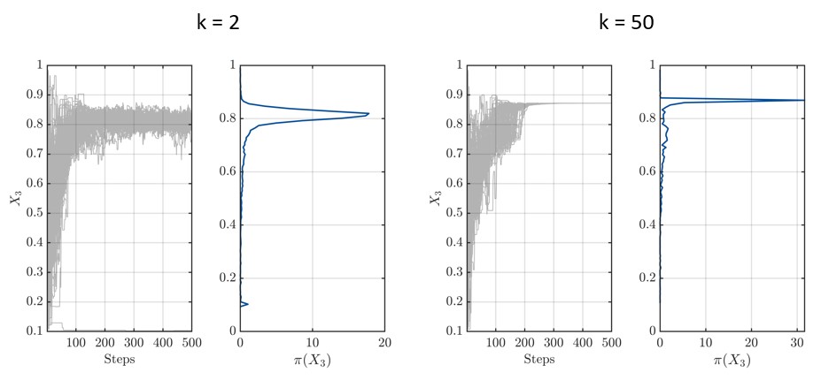
For k = 2 this corresponds to the classical normal distributions and the code runs as I expect. But as soon as I start to increase k to have an approximate uniform distribution the chains are approaching each other very close, which I do not understand.
Is there a mistake?
Best,
Marco
PS: I would like to share my entire script, but it seems, that I cannot upload it because I am a new user. I hope you have everything, otherwise please do not hesitate to ask.
Do you have reason to believe that your discrepancy model can be parameterized by a generalized Gaussian distribution? If so, could you elaborate on why?
It looks like what you observe can be expected from the likelihood definition. Because you consider a generalized normal distribution with a shape parameter k =50, the likelihood decays extremely fast from its ML point (i.e., its mode). Considering multiple measurements further amplifies this behavior.
Are you inferring the discrepancy variance sigma2 as well, or is it a constant? If you infer it as well, then your custom likelihood function is not correct, because the normalizing term - 1/2*logCdet only holds for a multivariate Gaussian, not the generalization that you are considering. In your case, it should depend also on the gamma function.
P.S.:
Maybe you could share the full custom-likelihood function? You should have the necessary rights now.
The reasons for doing this are to compare the results of the normal distributed likelihood function and the results of a uniform distributed likelihood function. The reason for choosing the generalized Gaussian distribution was to have a continuous function which is non-zero everywhere. But I am open for an alternative here.
Okay, thanks for the input. This may be the reason. Would you suggest then to choose an alternative to approximate the uniform distribution?
Yes, I am inferring sigma2 as well. Maybe like this? logLikeli_val = log(k) - log((2*gamma(1/k))^nOut2 * det(C)) - sum((abs((measurements(jj,:)-modelRuns(ii,:))*Cinv)).^k);
Here attached you can find the modified example: Examples.zip (16.1 KB)
I understand, but what is the motivation behind choosing a uniform distribution for the likelihood function? The likelihood function in model calibration typically follows from the assumed discrepancy model which, I assume, you choose as follows (i.e., additive discrepancy)
where you say that \mathbf{E} follows a (mutltivariate) uniform distribution. You thereby imply that data outside the support of the uniform distribution is impossible to observe. In the case of large k in the generalized normal distribution this still holds approximately. Is that correct?
Assuming that this is the case, and denoting the i-th model output by \mathcal{M}_i(\mathbf{x}) and the corresponding measurement by y^{(m)}_i, your likelihood function can be written as
The motivation for a uniform likelihood function is manifold: i) an informed distribution, pointing towards a most-likely value is difficult to defend based on the data we have and the type of model we use; ii) values outside the range of the uniform likelihood do not make physical sense and do not reflect the setup of our problem, iii) we do not have enough sources of discrepancy that would justify the central limit theorem, and last but not least iv) we would like to understand how much influence the choice of a likelihood shape has on the results we get (as we are not sure to have a multivariate gaussian)
Thank you for the correct formulation of the likelihood function. After double checking it, I implemented it in the code. However, it seems that this did not solve the problem that the chains are that close together. In the example sigma2 was given as a range [0\,\,300], then for the generalized gaussian to take the square root of that and multiply by two, to incorporate 95% of the normal distribution should not lead to that occurrence in my opinion.
Please find the updated version here: Examples_v2.zip (16.0 KB)