Can do Sobol's sensitivity analysis on arbitrary PCE?

Quynhchau · January 25, 2022, 5:23pm

Hi everyone.
I would like to ask question about PCE and also the sensitivity analysis. I have 800 output results based on 800 LHS samples with 7 random variables, running in FEM software. Based on the example PCE from existing data, the PCE metamodel was built and had a pretty good validation.
Below is my input data:

%% 4 - PROBABILISTIC INPUT MODEL
InputOpts.Marginals(1).Name = ‘DcRef’;
InputOpts.Marginals(1).Type = ‘Lognormal’;
InputOpts.Marginals(1).Moments = [3e-11 0.6e-11];

InputOpts.Marginals(2).Name = ‘mc’;
InputOpts.Marginals(2).Type = ‘Beta’;
InputOpts.Marginals(2).Parameters = [9.2944 52.6685 0 1];

InputOpts.Marginals(3).Name = ‘Uc’;
InputOpts.Marginals(3).Type = ‘Beta’;
InputOpts.Marginals(3).Parameters = [0.4437 0.1268 32e3 44.6e3];

InputOpts.Marginals(4).Name = ‘depth’;
InputOpts.Marginals(4).Type = ‘Gaussian’;
InputOpts.Marginals(4).Parameters = [0.04 0.01];
InputOpts.Marginals(4).Bounds = [0.01 inf];

InputOpts.Marginals(5).Name = ‘Xr’;
InputOpts.Marginals(5).Type = ‘Gaussian’;
InputOpts.Marginals(5).Parameters = [0.01 0.001];
InputOpts.Marginals(5).Bounds = [0 inf];

InputOpts.Marginals(6).Name = ‘Cfevn’;
InputOpts.Marginals(6).Type = ‘Lognormal’;
InputOpts.Marginals(6).Moments = [7.35 5.145];

% danh cho Cth
InputOpts.Marginals(7).Name = ‘Cth’;
InputOpts.Marginals(7).Type = ‘Gaussian’;
InputOpts.Marginals(7).Parameters = [2 0.4];

% Create an INPUT object based on the specified marginals:
myInput = uq_createInput(InputOpts);

%% 4 - POLYNOMIAL CHAOS EXPANSION (PCE) METAMODEL

% Select PCE as the metamodeling tool:
MetaOpts.Type = ‘Metamodel’;
MetaOpts.MetaType = ‘PCE’;
MetaOpts.Input = myInput;

%%
% Use experimental design loaded from the data files:
MetaOpts.ExpDesign.X = X;
MetaOpts.ExpDesign.Y = Y;

%%
% Set the maximum polynomial degree to 5:
MetaOpts.Degree = 1:5;

%%
% Provide the validation data set to get the validation error:
MetaOpts.ValidationSet.X = Xval;
MetaOpts.ValidationSet.Y = Yval;

%%
% Create the metamodel object and add it to UQLab:
myPCE = uq_createModel(MetaOpts);

%%
% Print a summary of the resulting PCE metamodel:
uq_print(myPCE)

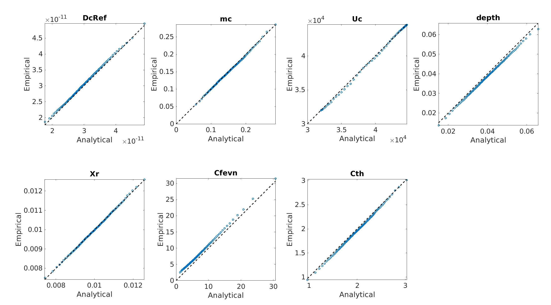
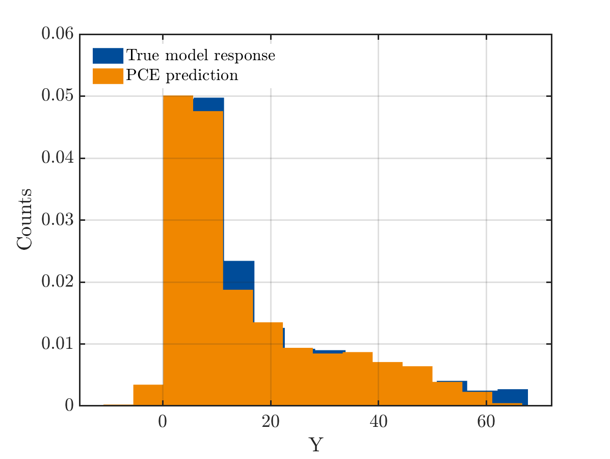
Below is the comparision of True model response and PCE model
uq_figure_1
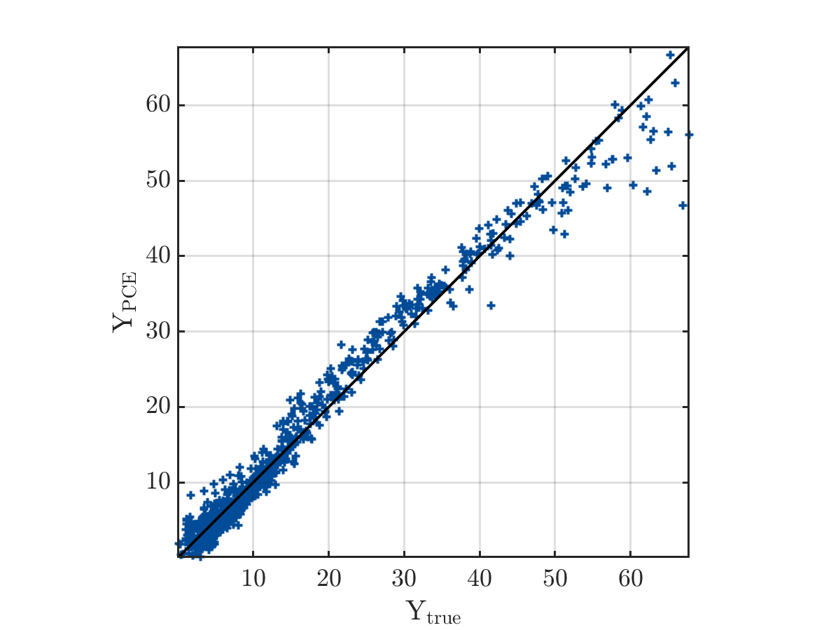
And the true output and PCE output
uq_figure_2

The result from UQlab is shown below:
------------ Polynomial chaos output ------------
Number of input variables: 7
Maximal degree: 3
q-norm: 1.00
Size of full basis: 120
Size of sparse basis: 64
Full model evaluations: 788
Leave-one-out error: 3.3906646e-02
Modified leave-one-out error: 4.5942902e-02
Validation error: 2.6473454e-02
Mean value: 34.6734
Standard deviation: 49.1539
Coef. of variation: 141.762%
--------------------------------------------------
PCE metamodel validation error: 2.6473e-02
PCE metamodel LOO error: 3.3907e-02

The mean value from UQlab is far from the mean value of real data, and as I read in some discussion available in UQlab forum, it does not mean I got the wrong PCE, but it is an arbitrary PCE. Therefore, the mean and the standard deviation of PCE model does not express the real mean and Std of the model. I have checked manually by comparing mean(YPCE) and mean(Yval) and they are the same, so I think the model is still right. My questions are:

Is there any way to transfer from arbitrary PCE to orthogonal PCE?
If not, can I do the Sobol’s sensitivity analysis on arbitrary PCE?
If I have the results of 800 simulations, can I use 800 samples for experimental design and also use the same 800 outputs for validation set?

I really appreciate any support and response from you.
Thank you so much.

styfen.schaer · January 26, 2022, 1:34pm

Dear Quynhchau

Can you refer to the post you mentioned?

Since you defined the distribution for all of your input variables, UQLab will automatically choose the polynomial family which is orthogonal to your input distribution. In your case, these are either Hermite or Jacobi.
The Sobol’s indices are computed from the PCE coefficients. As long as your PCE model is accurate you can compute them.
You can do this, and you even already have an error measure for it. See the leave-one-out cross-validation error in the output summary. However, if possible, you should validate your model with a separate data set. You can either split your existing data (for example, 80% for training and 20% for validation) or create a separate validation set. How you choose your validation set depends a bit on your problem. Are you interested in getting a good model for the entire input/output space, or are you interested in a specific domain of your input/output space? If the former, you can use standard random sampling (not LHS).

Perhaps @nluethen can tell you more about your PCE-specific questions.

Best regards
Styfen

giansteve · January 26, 2022, 1:52pm

Hi @Quynhchau,

I agree with @styfen.schaer. The polynomial functions are directly chosen from the PCE module of UQlab based on the distribution of your input parameters. In addition, if you prefer to impose particular polynomials on your PCE (which I discourage), you can do it with the following.

MetaOpts.PolyTypes = {'legendre','legendre','legendre'}; % dimension depending on the number of input parameters

The mean value from UQlab is far from the mean value of real data, and as I read in some discussion available in UQlab forum, it does not mean I got the wrong PCE, but it is an arbitrary PCE. Therefore, the mean and the standard deviation of PCE model does not express the real mean and Std of the model. I have checked manually by comparing mean(YPCE) and mean(Yval) and they are the same, so I think the model is still right.

Regarding the mean of the results produced from UQlab, I am afraid I did not get your question. Your data in the validation figure shows a non-normal probability distribution. Therefore, it is inaccurate to talk about the mean value. From your pictures, the two datasets look in good agreement, in my opinion. Maybe you could compare the median values of the distributions. It would be best to compute this value independently, because UQlab does not show it.

I hope I was clear. Let me know if something is still hazy.

bsudret · January 26, 2022, 3:55pm

Dear @Quynhchau

Thanks for your detailed questions. Some answers have been given already. Let me add some comments.

Is there any way to transfer from arbitrary PCE to orthogonal PCE?
As it was said above, as your inputs are independent the polynomials are automatically selected to be orthogonal to each input distribution. Thus you can define a sensitivity analysis right after defining the PCE, and Sobol’ indices will be computed from the PCE coefficients.
If I have the results of 800 simulations, can I use 800 samples for experimental design and also use the same 800 outputs for validation set?
A validation set must be independent from the training set. If you use the same points, you would estimate the so-called empirical error, which usually underestimate the true mean-square error. As suggested by @styfen.schaer, if you only have these 800 points in total and cannot generate more, you could split into 80% for training, 20% for validation.
This is, however, not useful in practice: the reported leave-one-out error (resp. modified LOO) “mimics” the computation of a mean-square error without the need of an independent validation set. This way you use all your data for training, and still get an error estimate that makes sense. See the UQLab user manual – Polynomial chaos expansion page 7-8.

Finally, in your input file, you use the degrees MetaOpts.Degree = 1:5. I think you could increase the maximal degree up to 10, and add also a search on the so-called q-norm truncation scheme: MetaOpts.TruncOptions.qNorm = 0.5:0.1:1. This will generate more candidate bases (and corresponding LAR analyses) and you may get in the end a sparse PCE that is more accurate that would have obtained so far.
No guarantee though … My comment is based on the fact that I would expect a better accuracy in your case with d=7 parameters and 800 points in your experimental design, especially the latter has been sampled using LHS.

Good luck!
Best regards

bsudret · January 26, 2022, 3:57pm

PS: Your output distribution looks very skewed, and has a large coefficient of variation. Another trick that may help, if your output y is positive in nature: try to surrogate \log y, i.e. build a PCE using the log-outputs.

Quynhchau · January 26, 2022, 4:01pm

Thank @styphen.schaer for your reply.
Yes, I think my PCE model is good enough now, excepting that maybe I need more data to get smaller LOO error, that should be <0.01.

I am interested in getting the good model for the entire input/output space. But the computational cost is very high so I have to choose the LHS method.

For PCE question, I know UQlab will automatically define the polynomial family of my input distribution, also create the optimized PCE. However, I wonder that in the Manuals_PCE, it is said that the PCE can be post-processed to obtain further information about the quantities of interest, including moments of a PCE and sensitivity analysis. This sentence is true in the case of example PCE METAMODELING: TRUSS DATA SET, when the mean value of the PCE reads: µPC = y0. The mean shown on output summary (y0) equals to the mean of data set.

However, in my case, y0 in the function M(X)(PCE model) can not be read as the mean value, because my PCE is an arbitrary PCE. And as I read about Sobol’s indices sensitivity analysis, the Sobol’s decomposition is defined as:
Capture
and f0 is constant and equal to the expected value of f(x). In the case my PCE model is not a basic model, can I do the Sobol’s indices sensitivity on my aPCE.
Sorry I ask this question again, but I just want to make sure how UQlab works in this case.

Thank you and looking forward to hearing from you!
Regards,
Quynh Chau

Quynhchau · January 26, 2022, 4:10pm

Thank @bsudret for your detailed reply.

I have written my response and did not notice your answer was coming. But it is really helpful.
For your trick, it is interesting to know that. Could you please explain more how to build a PCE using the log-outputs. Actually, my output results is expected to follow the lognormal distribution and have no positive value in nature.

Thank you so much for your support.
Regards,
Quynh Chau

styfen.schaer · January 26, 2022, 5:29pm

Dear @Quynhchau

The fact that the first two statistical moments can be calculated from the PCE coefficient is due to the orthogonality of the polynomials. So even if you use arbitrary polynomials, you should still be able to calculate the mean and variance from the coefficients. However, you are not using arbitrary polynomials in the problem you showed.
Can you refer to the passages/posts/examples that may cause this confusion?

What @bsudret meant is the following: If y is the output of you experimental design, then you compute y_{log}=\log y. Now you build your PCE on y_{log}. When you now apply your PCE to new data you will obtain the prediction \hat y_{log}. So don’t forget to apply the corresponding exponential (inverse of the logarithm) to get your desired prediction \hat y.
If your output is to follow a lognormal distribution, your values should have only positive values. This is the nature of a lognormal distribution, that the values are positive. Hope that makes sense to you.

Best regards
Styfen

Quynhchau · January 26, 2022, 5:56pm

Thank @styfen.schaer
I want to make my example clear for you. When I run 800 simulations in Fem software and get 800 outputs, the mean value of data set is 15.69. By running the PCE in UQLab, as I expected to see in the output summary is that, Mean value is around 15.69 (and y0 in PCE model is also the mean of data). In the example of UQlab, I have checked the original data and realized that the mean of experimental design set is approximately with Mean value exported by UQlab. But for my case the result is:
Number of input variables: 7
Maximal degree: 3
q-norm: 1.00
Size of full basis: 120
Size of sparse basis: 64
Full model evaluations: 788
Leave-one-out error: 3.3906646e-02
Modified leave-one-out error: 4.5942902e-02
Validation error: 2.6473454e-02
Mean value: 34.6734
Standard deviation: 49.1539
Coef. of variation: 141.762%
The mean value from UQlab, which is obtained from the first coefficient of MPC(x) is 34.67, this result is not meaningful to express the mean value of the model. But I can calculate the mean and variance based on the available PCE model. Maybe I get misunderstanding that for PCE model, we always can get the y0 as the mean value. Please fix it if I am wrong.

Thats why I think my PCE model is an arbitrary PCE. Even though, thanks to all of your comments, I concluded that I still do the Sobol’s indices sensitivity on my PCE model. And I should improve the accuracy for my case first by adding some modifications for it.
Thank you,
Regards,
Quynh Chau

ste · January 29, 2022, 8:46pm

Hi @Quynhchau
thanks for your post.

Just my 2 cents: “arbitrary PCE” only means that the polynomials are constructed orthogonal wrt to your input distributions, whatever they are. It has no consequence on the interpretation of the coefficients and whatnot. So the first coefficient y0 should always converge to the true mean of your model.

What concerns me is that according to the output you just pasted, PCE returns a mean value that is approximately 2x the mean value of your experimental design. This is almost impossible in practice, which in my eye means that there is some inconsistency in what you are doing.
The only way that comes to my mind to create such a situation is when the distributions you used to sample your 800 experimental design points are different than those you use to construct the PCE.
If you are sure instead that everything is correct, please either share here your code and experimental design, or contact us at uqlab@ethz.ch, so that we can find the root of this inconsistency.

Cheers
stefano

Quynhchau · February 3, 2022, 4:19pm

Thank @ste for your clear response.
Yes, what you said was exactly what I wondered and couldn’t find the suitable answer for it. I am quite sure that my code and experimental design is correct. I will upload necessary files here and hope you can help me to find the root of the inconsistency.
uq_Maincode.zip (90.1 KB)
Some information about my inputs

Variable	Mean	COV	Distribution
D_(ref )	3 x 10-11 m2/s	0.20	Log-normal
U_c	41.8 kJ/mol	0.10	Beta on [32,44.6]
m_c	0.15	0.30	Beta on [0,1]
C_th	0.5 wt% cement	0.20	Normal
C_fevn	7.35 kg/m3	0.7	Log-normal
Depth	40 mm	0.25	Normal (truncated at 10 mm)
X_r	10 mm	0.1	Normal (truncated at 0 mm)

I am really looking forward to receiving your response.
Thank you so much!

ste · February 4, 2022, 11:27am

Hi @Quynhchau
thanks for sharing your data.

In short, as @xujia and myself mentioned in the post, the problem lies in a discrepancy between your training set X and the distributions you quote and use in the code.
In short, there are several problems with the data you sent:

Variable 6 in your script (C_fevn) is shifted to the right of approx 1.2 wrt to your tabulated distributions, as well as on the distributions specified on the script. Its mean value is approx. 8.5 vs the expected 7.35
Variable 4 (depth) does not respect the bounds you requested (its min value is 0.0088 > 0.010).

In general, you can see a lot of issues by looking at the following qq plots of your input variables:

As you can see, Cfevn from your data has a large shift wrt the expected values from the distributions you provided (in all plots x is the expected quantile, y is the empirical quantile from your experimental design). Some other variables, e.g. Xr or Mc, look mostly ok. But you can see smaller shifts/deviations for depth, cth and others.

While those shifts may not look that important, when you analyze the model response vs the inputs, you realize that this may have an enormous importance on your model output. The following image highlights in red the input combinations that belong to an output quantile of 0.99 and higher:
pmatrix

What you can see is that all the high values of the model response Y correspond to low values of Cfevn. Because Y is extremely skewed, a shift in Cfevn towards larger values corresponds to a very significant decrease in the sample mean. Here’s an x vs y plot to show you the tails of Y:

Basically your input sample is biased with respect to the input distributions you provided, which causes your output to have a much lower mean than what you would expect. If you see the above image Y vs. X, a factor of 2 on the estimated mean seems very realistic.
The mean estimate from PCE is correct given the input distributions: if you resample a new set of points from the input, the mean value will be very close to its constant term.

TL:DR, your experimental design X does not belong to the same distributions you specified in UQLab, which causes the corresponding model response Y to have a much smaller tail, hence severely underestimating the actual mean value of your response.

As to why your X is so different than the distributions you specify, I do not know. We could not reproduce any of this bias with UQLab, which means that either you used UQLab to sample your experimental design with different distributions, or you used some other method.

I hope this makes sense!
Best
stefano

Quynhchau · February 7, 2022, 5:05pm

It is an extremely great answer. Thank you so much.
Now everything is clear for me.
Just want to explain what happened with my input to make this topic clear for everyone. I run 1000 LHS samples in FEM software, and because of the constraint of FEM software memory, 20% of output exceed the time service of the structure, so I did not use those results. That means I have deleted the input sample relating to unused results, and keep 788 valid results.
Your clear explanation remind me about what I did because I thought there is no problem with my data. But I made mistake :). Actually, as you said, the PCE model did a good job because it may give me the right mean of data even I could not get it from the original data. So it is interesting to know more about that.
Again, thank you so much for your support.
Regards,
Quynh Chau

lqz · May 21, 2022, 8:33am

Hi,Quynchau, I am a student from Sun Yat-Sen University. This problem is exactly what I am working on. I thibk that the theory of aPCE is different from that of the traditional PCE, so coefficients cannot be directly used for post-processing. I think it is possible to build aPCE as a proxy model based on the data and then use Mc-sobol for sensitivity analysis.

Best regards
Qizhe Li