Problem statement
Heat transfer models are ubiquitous in engineering disciplines. They are typically used to model the heat evolution in various mechanical components, structural members and systems. In civil engineering, heat transfer models are utilized to simulate the behaviour of structures exposed to fire. These models typically consist of complex finite element simulations that are then used to determine whether a structure is safe in the case of a fire event.
To accurately simulate the whole structure, the thermal material properties of the structural members and more specifically, the thermal properties of the insulation materials need to be determined. Heat insulation is often provided by gypsum boards that are added to structural members to shield them from fire-induced heat exposure.
During the charring of the gypsum boards, processes that are not explicitly considered in the employed engineering models take place. To nonetheless capture these processes, the materials are modelled with temperature-dependent effective material properties. These thermal properties are the material density \rho(T), the thermal conductivity \lambda(T), and the specific heat capacity c(T) all varying with the temperature T.
In this post, I will outline an approach to determine these properties by calibrating a transient heat transfer model using available measurements of the heat evolution in a small number of experiments. We carry out the calibration using the Bayesian inference framework. This allows the combination of the few available experimental observations with the knowledge available from prior calibration attempts and expert judgment.
Methods and tools
Computational model and measurements
We start out with a set of transient temperature measurements \mathcal{Y} = \{\mathbf{y}^{(i)}\}_{i=1}^M collected at discrete time steps. These measurements were obtained from placing a gypsum board in a furnace and recording the heat evolution at a certain distance to the exposed surface across multiple locations of the specimen over time (see Figures 1 and 2).
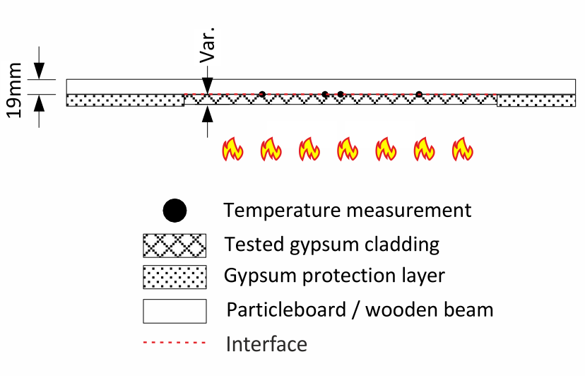
Figure 1 – Sketch of the used setup for testing the gypsum cladding.
The heat evolution is modelled with a 1D transient finite element simulation that takes as an input the temperature dependent material properties and returns the predicted temperature at one location.
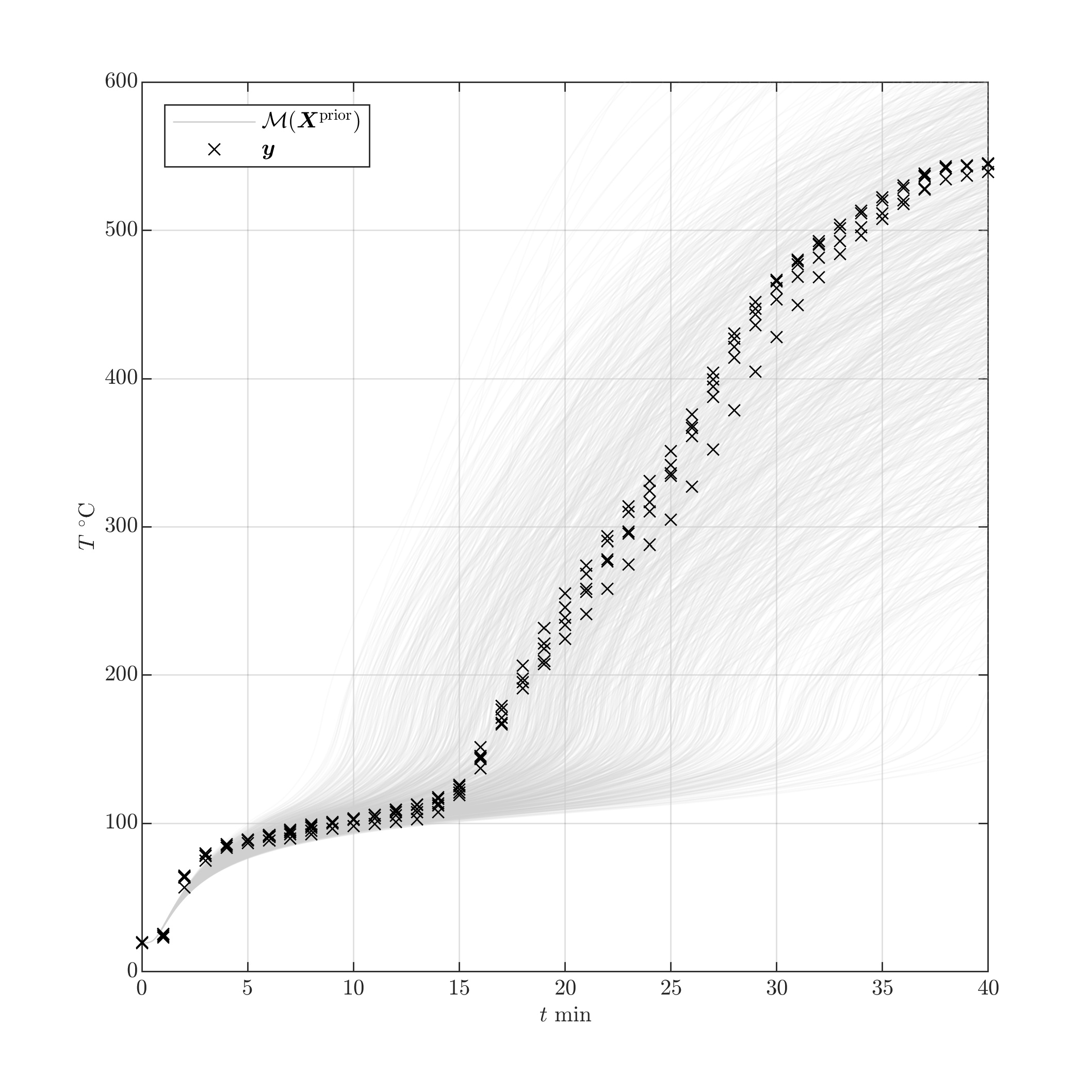
Figure 2 – Non-calibrated model predictions and available measurements.
To calibrate these properties, we parametrize them using a set of model parameters \mathbf{X}=(X_1,\dots,X_6). One set of parameters uniquely defines a material property curve through the red knots seen in Figure 3.
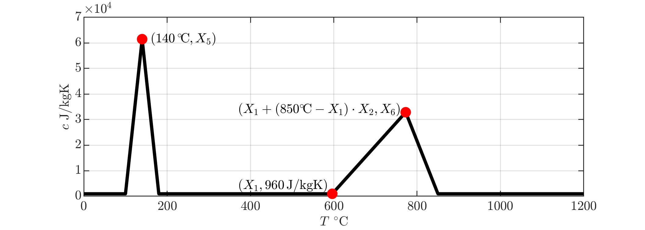
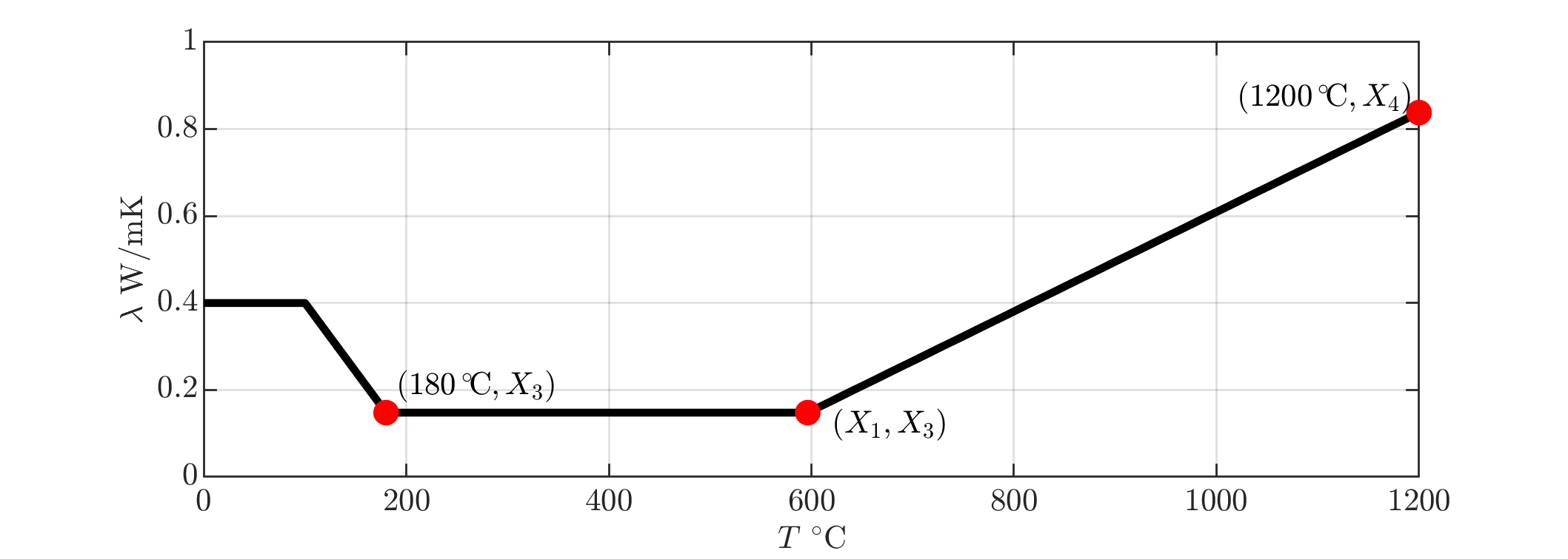
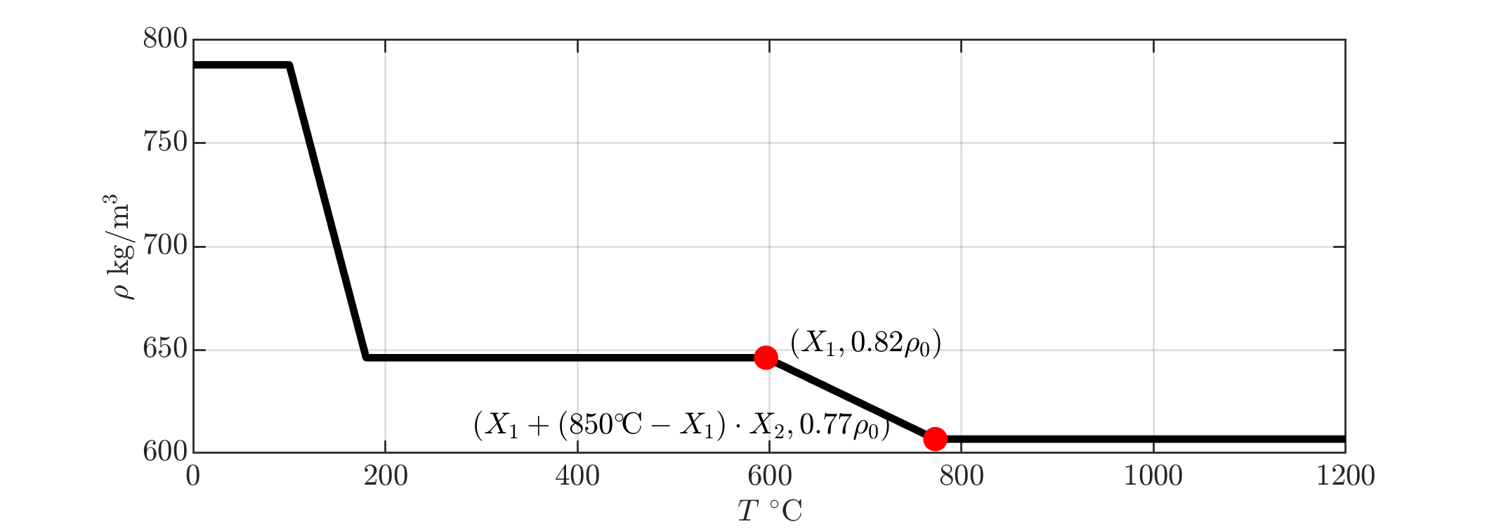
Figure 3 – Parametrization of the temperature-dependent effective material properties (from top to bottom: specific heat capacity, thermal conductivity, material density).
For a given parameter vector the finite element model \mathcal{M} then returns the simulated heat evolution at the measurement location in N=401 discrete time steps:
Bayesian inference framework
To determine the model parameters that best describe the observed temperature evolution, we employ the Bayesian inference framework (Nagel and Sudret, 2016; Wagner et al., 2018). It is a statistical inference method that is especially useful for problems with few available measurements. We assume that the parameters are realizations of a random variable distributed according to a prior distribution \mathbf{X}\sim\pi(\mathbf{x}). In practice a uniform distribution between reasonable bounds is often assigned to each parameter. This prior distribution is then updated to reflect the new information about the parameters obtained from the experimental observations \mathcal{Y}.
Updating these probabilities can be expressed through Bayes’ theorem as follows:
where \mathcal{L}(\mathbf{x};\mathcal{Y}) is the likelihood function of the parameters given the observations \mathcal{Y}. It represents how likely a particular value of \mathbf{x} of the input parameters is with respect to the available data \mathcal{Y}. The posterior distribution \pi(\mathbf{x}\vert\mathcal{Y}) expresses the updated parameter distribution which results from the combination of the prior knowledge and the data. The maximum of this distribution is often used in calibration problems to denote the most likely parameter value. It is called maximum a posterior (MAP) estimator and denoted by \mathbf{x}^{\mathrm{MAP}}.
Computing the posterior distribution
The posterior distribution can usually not be computed in closed-form. Instead, it is a common practice to sample from it. One widely used technique for that is Markov chain Monte Carlo (MCMC) simulation (Gelman et. al., 2013).
A shortcoming of any sampling-based method (like MCMC) is the necessity to repeatedly evaluate the likelihood function, which contains the evaluation of the computational model \mathcal{M}. The high computational cost associated with carrying out tens of thousands of finite element runs can be alleviated by initially constructing a surrogate model from a set of model runs and further using this surrogate in lieu of the original model in the MCMC simulation.
In this case study we use a combination of polynomial chaos expansions (PCE) with principal component analysis (PCA). This combined surrogate modelling technique allows to efficiently surrogate models with multiple output dimensions by reducing the dimensionality of the model output (in our case, the temperature time series) from N to P\ll N.
Results
Using the affine-invariant ensemble sampler (Goodman and Weare, 2010), we generate a sample distributed according to the posterior distribution. Figure 4 shows the resulting posterior material properties along with the MAP estimator and Figure 5 shows the model predictions and the measurements used for calibration. From these figures, we can clearly see that the posterior predictions closely match the available measurements.
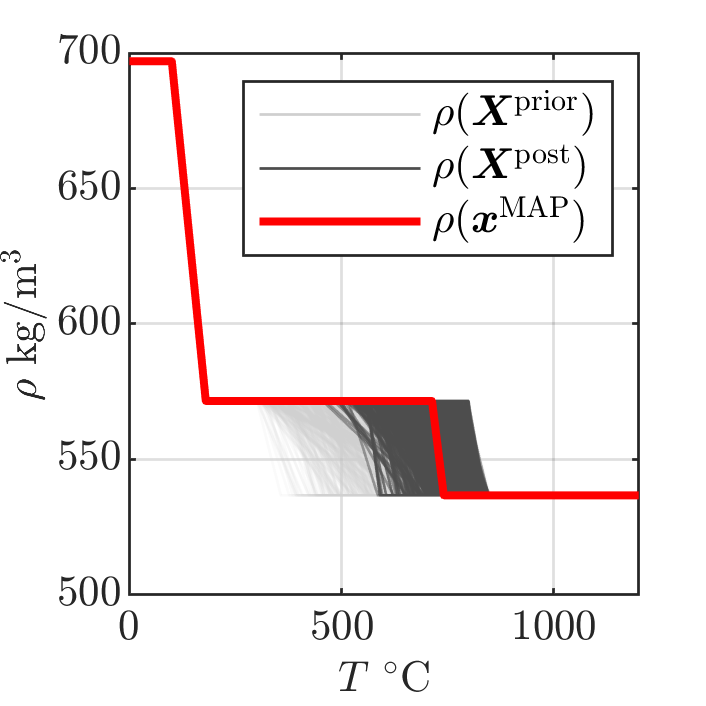
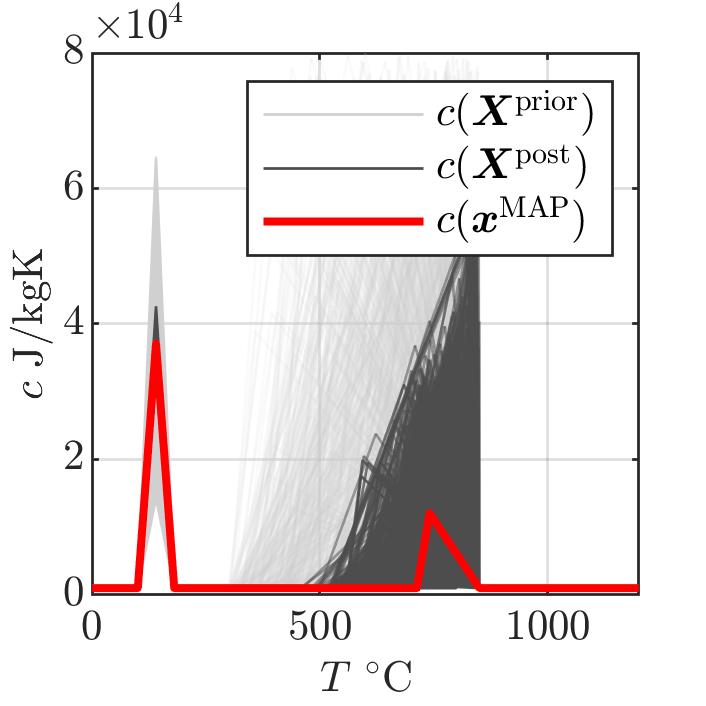
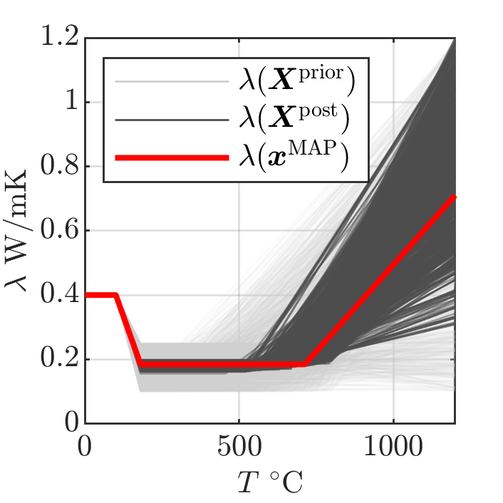
Figure 4 – Prior and posterior material properties and the MAP estimator \mathbf{x}^{\mathrm{MAP}}.
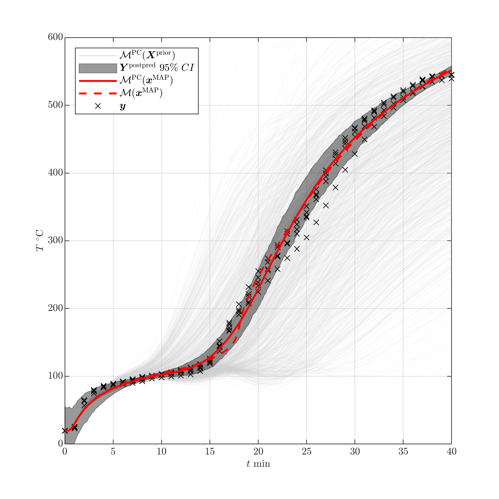
Figure 5 – Prior and posterior predictions of the surrogate model \mathcal{M}^{\mathrm{PC}}, MAP predictions and the data \mathbf{y}^{(i)}.
Conclusion
As opposed to pure pointwise calibration strategies, the Bayesian procedure delivers the full distribution of the posterior model parameters. This distribution can be used to provide confidence intervals on the calibrated parameters on top of the best estimate maximum a posteriori values.
Notes on uncertainty quantification (UQ) tools
All the tools I used for the analysis presented in this post are available in UQLab. More specifically, the surrogate model was created with the Polynomial chaos expansions module and the calibration was conducted with the Bayesian inversion module using the affine-invariant ensemble sampler and the user-defined likelihood option.
References
- A. Gelman, J.B. Carlin, H.S. Stern, D.B. Dunson, A. Vehtari, and D.B. Rubin, Bayesian Data Analysis, Texts in Statistical Science, New York: CRC Press, 2013. DOI:10.1201/b16018
- J. Goodman and J. Weare, “Ensemble samplers with affine invariance” Communications in Applied Mathematics and Computational Science, vol. 5, no. 1, pp. 65–80, 2010. DOI:10.2140/camcos.2010.5.65
- J. Nagel and B. Sudret, “A unified framework for multilevel uncertainty quantification in Bayesian inverse problems” Probabilistic Engineering Mechanics, vol. 43, pp. 68–84, 2016. DOI:10.1016/j.probengmech.2015.09.007
- P.-R. Wagner, R. Fahrni, M. Klippel, and B. Sudret, “Bayesian inversion for the calibration of fire experiments on insulation panels”, In the Proceedings of the 19th IFIP WG-7.5 conference on Reliability and Optimization of Structural Systems, ETH Zurich, Zurich, Switzerland, June 26–29, 2018. DOI:10.3929/ethz-b-000304641
- P.-R. Wagner, J. Nagel, S. Marelli, and B. Sudret, “UQLAB user manual – Bayesian inference for model calibration and inverse problems”, Report UQLab-V1.2-113, Chair of Risk, Safety & Uncertainty Quantification, ETH Zurich, 2019. URL