hello everyone
My uncertainty quantification problem doesn’t have a definite function relationship between input and output because the output is calculated by CFD based on corresponding input values. Which means Unable to create a “model” as defined in uqlab. So, I can’t define a model and have to use the manual input data method(existing data). I want to input existing data and still use Gaussian quadrature to calculate the PCE coefficients. I found that there is a significant error in the computation, but theoretically, the accuracy of a fourth-order PCE should be sufficient to predict the uncertainty quantification (UQ) problem in our field. How can I get the correct results?
- List item
Research problem Description: Uncertainty quantification for a one-dimensional normal distribution N(0,0.16672) input variable.( Just preliminary research, there are high-dimensional problems to be addressed later.")
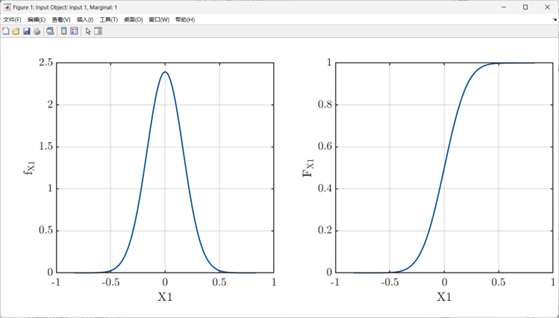
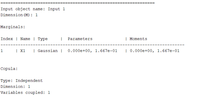
My input variables: The input variable is one-dimensional and follows a normal distribution N(0,0.16672).
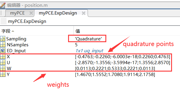
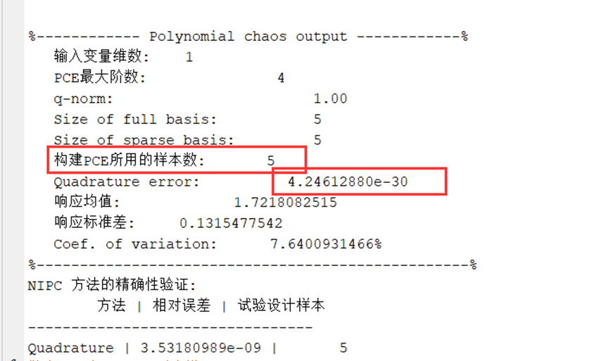
I selected a PCE degree of 4, so there are 5 sample points according to Gaussian quadrature .
I noticed in the manual:

For projection-based PCE, the experimental design is determined by the choice of quadrature scheme and degree. Since I chose a PCE degree of 4, there are 5 sample points, all of which are specific points.
For my input variable distribution, using Gaussian quadrature, the experimental design is determined by the choice of quadrature scheme and degree.
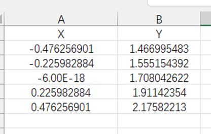
My input data is in Excel, where X is obtained through the quadrature scheme and degree based on the existing distribution, and Y is obtained through CFD for each data point of X.
After calculating like this, the error is very large and cannot achieve good results.
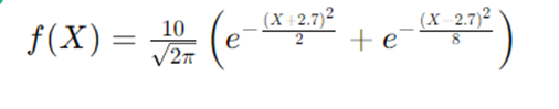
So I chose a one-dimensional model function for testing and found the problem
by defining the model.
clearvars
rng(100,'twister')
uqlab
%% 2 - Model Computation
% Define MATLAB expression string
modelopts.mString = '10/sqrt(2*pi) * (exp(-(X+2.7).^2/2) + exp(-(X-2.7).^2/8))'; % One-dimensional function
modelopts.isVectorized = true;
myModel = uq_createModel(modelopts);
%% 3 - Define Input Random Variable Model
InputOpts.Marginals(1).Type = 'Gaussian';
InputOpts.Marginals(1).Parameters = [0 0.1667];
% Create an input object based on specified marginal distributions
myInput = uq_createInput(InputOpts);
uq_print(myInput)
uq_display(myInput);
%% 4 - Polynomial Chaos Expansion (PCE) Metamodel
% Choose PCE as the metamodel tool in UQLab:
MetaOpts.Type = 'Metamodel';
MetaOpts.MetaType = 'PCE';
MetaOpts.FullModel = myModel;
MetaOpts.Method = 'Quadrature';
MetaOpts.Degree = 4;
%%
myPCE = uq_createModel(MetaOpts);
% Print the computed PCE report:
uq_print(myPCE)
% Visualize the spectrum of nonzero coefficients obtained
uq_display(myPCE)
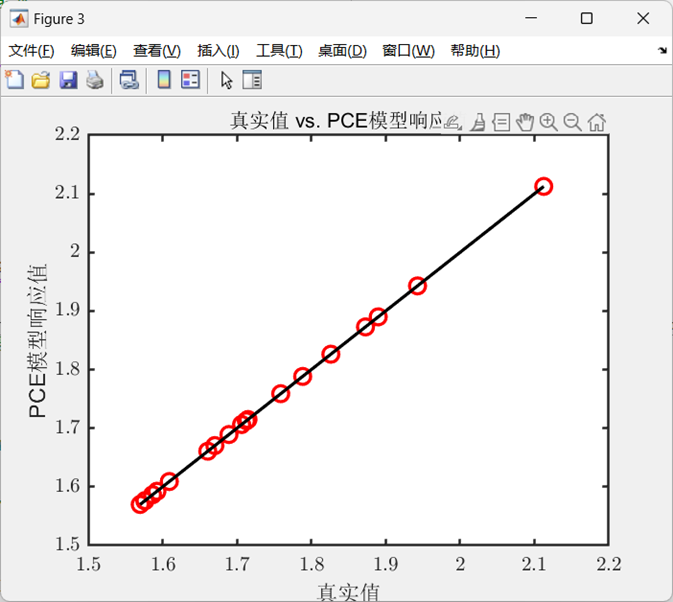
%% 5-2-1 NIPC Response vs. True Value Plot Validation
figure;
uq_plot(Yval, YQuadrature, 'ro', 'MarkerSize', 10, 'LineWidth', 2, 'MarkerFaceColor', 'none'); % Plot PCE model response values, using red
hold on
uq_plot([min(Yval) max(Yval)], [min(Yval) max(Yval)],'k')
% Set figure properties
title('True Value vs. PCE Model Response');
xlabel('True Value');
ylabel('PCE Model Response');
grid;
hold off;
% Compute validation errors
fprintf('NIPC Method Accuracy Validation:\n');
fprintf('%10s | Relative Error | Experimental Design Samples\n', 'Method');
fprintf('---------------------------------\n');
fprintf('%10s | %10.8e | %7d\n', MetaOpts.Method, mean((Yval - YQuadrature).^2)/var(Yval), myPCE.ExpDesign.NSamples);
%% 5 - NIPC Method Accuracy Validation
% Create a validation sample of size $10^4$ from the input model:
Xval = uq_getSample(20);
% Evaluate the true values at the sample points:
Yval = uq_evalModel(myModel,Xval);
% Generate the response values of the created PCE model at the sample points:
YQuadrature = uq_evalModel(myPCE,Xval);
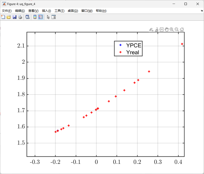
%% 5-5-3 NIPC Input vs. Predicted Values Plot (Applicable for One Dimension)
% Plot scatter plot of true values vs. predicted values:
uq_figure
%
uq_plot(Xval, YQuadrature, 'b+')
hold on
uq_plot(Xval, Yval, 'r+')
legend('YPCE', 'Yreal');
From the results, it can be seen that only five samples were used, and the constructed error is very small.
However, using the same computational method and providing only five data points without defining a model have big error.
clearvars
uqlab
%% 2 - Obtaining Dataset
% Read data from Excel
filename = 'E:\UQ\UQLab_Rel2.0.0\uq_test37\uqdata.xlsx';
% Read data from Excel file
data = xlsread(filename);
% Assign data to X and Y
X = data(:, 1); % Save the first column of data to X
Y = data(:, end); % Save the last column of data to Y
% Save data to MAT file
save('angle.mat', 'X', 'Y');
%%
% Read experimental design dataset file and store the content in a matrix:
load(fullfile('angle.mat'), 'X', 'Y');
%%
%% 3 - Input Model
%
% Since PCE requires the selection of polynomial bases,
% a marginal distribution of the probability input model needs to be defined.
% Specify the marginal distribution of the probability input model:
InputOpts.Marginals(1).Type = 'Gaussian';
InputOpts.Marginals(1).Parameters = [0 0.1667];
%%
% Create an INPUT object based on the specified marginal distribution:
myInput = uq_createInput(InputOpts);
%% 4 -1 Polynomial Chaos Expansion (PCE) Metamodel
%
% Choose PCE as the metamodel tool:
MetaOpts.Type = 'Metamodel';
MetaOpts.MetaType = 'PCE';
%%
% Use the experimental design loaded from the data file:
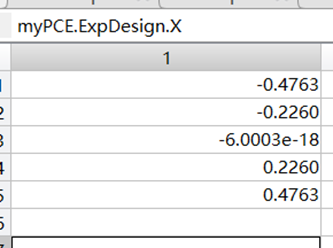
MetaOpts.ExpDesign.X = X;
MetaOpts.ExpDesign.Y = Y;
MetaOpts.Method = 'quadrature';
MetaOpts.Degree = 4;
myPCE = uq_createModel(MetaOpts);
%%
% Provide validation dataset for validation error calculation:
Xval = uq_getSample(200);
%
%%
% Print summary information of the generated PCE metamodel:
uq_print(myPCE)
%% 4 -2 PCE Validation
%
% Evaluate the PCE metamodel at validation set points:
YPCE = uq_evalModel(myPCE,Xval);
uq_figure
%
uq_plot(Xval, YPCE, 'b+')
hold on
uq_plot(X, Y, 'r+')
legend('YPCE', 'CFD');
hold off
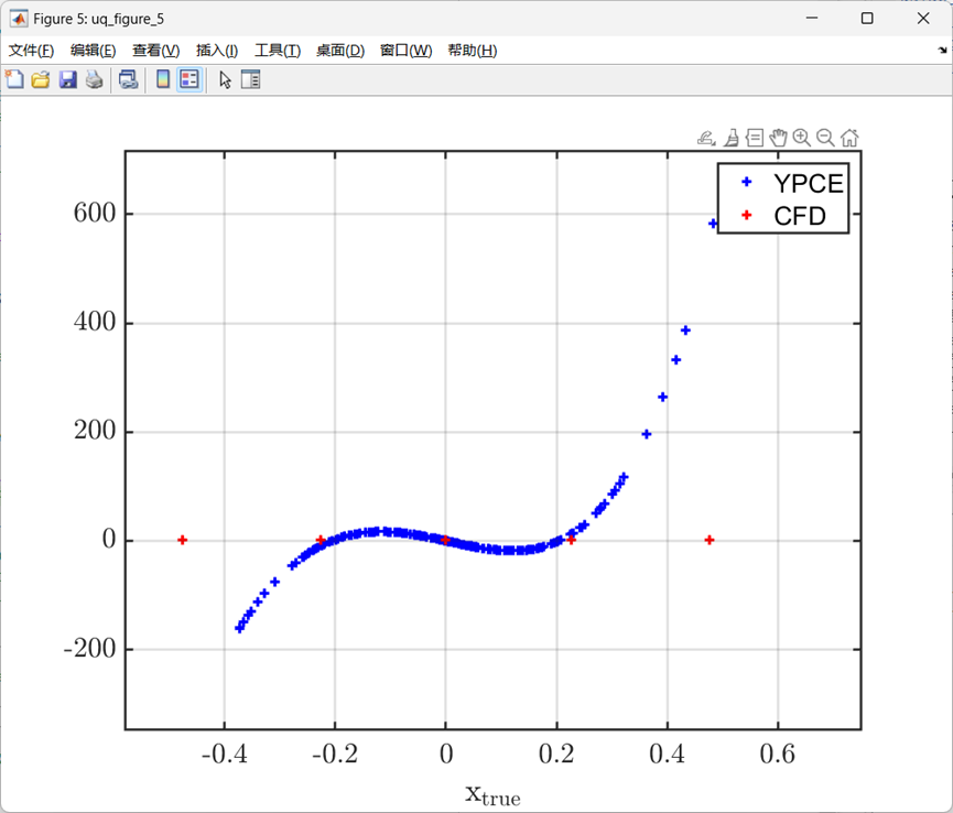
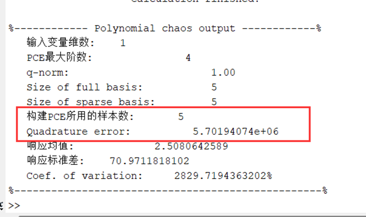
You can see that the error is very large.
Data display in E:\UQ\UQLab_Rel2.0.0\uq_test37\uqdata.xlsx
my questions are:
- Can I Calculating the PCE coefficients with Gaussian quadrature using existing data?
- If yes, how should I proceed?
Thanks in advance