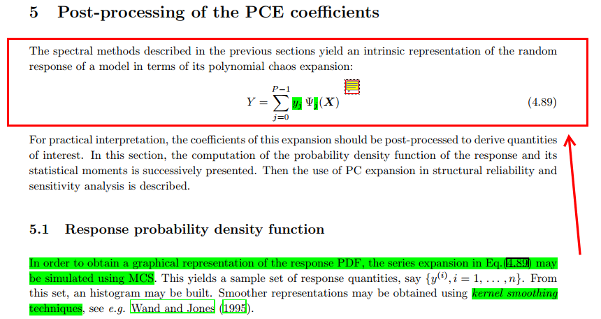
The code I have is based in Emil Brandt Kærgaard thesis (DTU), it is a Multidimensional Collocation Method using a Gauss-Legendre sparse grid, and is perfectly calculating the mean and variance as follows:
Either way, I don’t seem to be able to understand how to assemble the surrogate in this multivariate case, it is getting really hard to progress. I have been reading materials from Bruno Sudret (mainly Blaise Pascal monograph), the aforementioned thesis (DTU), and the book by Dongbin Xiu (numerical methods for stochastic computation).
Would you please suggest a beginner source for this matter, or even a tip? All comments are much appreciated!
Maybe you can be more specific about what you already have and what is missing and where exactly you are stuck.
And do I understand correctly that you are trying to implement PCE from scratch? Is there any reason to do this? There are powerful implementations (UQLab, but also many others) that are well tested and already offer very advanced state-of-the-art features.
I have previously used UQlab in some tests, it is indeed a wonderful tool. I am trying to implement my version of PCE so I can fully understand the method (which is very confuse in my opinion, especially the multivariate version).
To sum it up:
-a toy problem is solved in time domain by Newmark - 1gdl mass-spring-damper.
-the toy problem is evaluated with very specific sparse grid points as input (scaled to the input dimensions and uncertain interval).
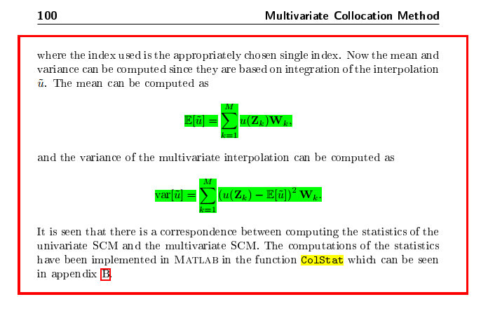
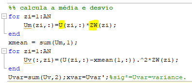
-the resulting displacement signals, U, are then used to obtain the mean (xmean) and variance (xvar) of the displacement in each time step. ZW are the weights of the grid points, and AN is the total number of grid points:
I have tested this code against Monte Carlo Simulation in different problems, and it seems correct.
From this, I was trying to figure out how to build the surrogate PCE for a given time in the signal, so i can build the PDF. Can you confirm that this is done by means of the basis polynomials, in this case Legendre polynomials, U and ZW?
I will provide my matlab files bellow, in case you want to check out. This code was done based on Emil Brandt Kærgaard thesis (DTU), as mentioned previously. The files regarding the Gauss-Legendre sparse grid were downloaded from this link.
Thank you again for your reply, it is much appreciated.
I’m afraid I don’t understand exactly where you’re stuck. If your goal is to better understand PCE by implementing a basic version of it (which I think is a good idea), then I recommend using a simple case study (like this one: https://www.uqlab.com/uqlink-c-simply-supported-beam) and finding the coefficients using least squares. This is also something we let students start with to get familiar with surrogate modeling and PCE in particular. If it comes to your actual case study, I would then switch to a software of your choice offering a more sophisticated and versatile implementation of PCE.
If you feel that such a simple case study would be helpful, I can provide some sample code as a guidance.
This is a minimalist implementation of a multivariate PCE applied to a simple case study. The same PCE is also implemented in UQLab for comparison. It is only for uniformly distributed random variables (Legendre polynomials) and the basis is a total degree basis.
It may be helpful to look at the manual regarding the terminology :
I hope this helps you to move forward!
See code here
%% Setup
clearvars
rng(1, 'twister')
uqlab

%% Define computational model
ModelOpts.mFile = 'uq_ishigami';
myModel = uq_createModel(ModelOpts);

%% Define input
for ii = 1:4
    InputOpts.Marginals(ii).Type = 'Uniform';
    InputOpts.Marginals(ii).Parameters = [-1, 1];
end
myInput = uq_createInput(InputOpts);

%% Generate training and validation date
N_train = 2e2;
X_train = uq_getSample(myInput, N_train);
Y_train = uq_evalModel(myModel, X_train);

N_val = 1e4;
X_val = uq_getSample(myInput, N_val);
Y_val = uq_evalModel(myModel, X_val);

%% Fit custom PCE model
degree = 5;
myPCE = create_pce(degree, X_train, Y_train);
Y_pce1 = eval_pce(myPCE, X_val);

%% Fit PCE model using UQLab for comparison
MetaOpts.Type = 'Metamodel';
MetaOpts.MetaType = 'PCE';
MetaOpts.Method = 'OLS';
MetaOpts.degree = 5;
MetaOpts.PolyTypes = {'Legendre', 'Legendre', 'Legendre', 'Legendre'};
MetaOpts.ExpDesign.X = X_train;
MetaOpts.ExpDesign.Y = Y_train;

uqPCE = uq_createModel(MetaOpts);
Y_pce2 = uq_evalModel(uqPCE, X_val);

%% Validation and comparison plot
figure
scatter(Y_val, Y_pce1, 15, 'filled', 'MarkerFaceAlpha', 0.5)
hold on
scatter(Y_val, Y_pce2, 10, 'filled', 'MarkerFaceAlpha', 0.5)
xlabel('Y_{val}')
ylabel('Y_{PCE}')
legend('custom', 'UQLab')

%% PCE implementation
function pce = create_pce(degree, X, Y)
    %
    % Fit PCE of total degree 'degree' to input 'X' and output'Y' using least-squares
    %
    alphas = create_alphas(size(X, 2), degree);
    Psi = compute_psi(X, alphas);
    coef = pinv(Psi' * Psi) * Psi'*Y;
	pce = struct(degree=degree, alphas=alphas, coef=coef);
end

function Y = eval_pce(pce, X)
    %
    % Evaluate fitted PCE model at inputs 'X'
    %
    Psi = compute_psi(X, pce.alphas);
    Y = Psi * pce.coef;
end

function Psi = compute_psi(X, alphas)
    %
    % Compute regression matrix for inputs 'X' and basis 'alpha'
    %
    Psi = ones(size(X, 1), size(alphas, 1));
    for jj = 1:size(Psi, 2)
        for kk = 1:size(alphas, 2)
            Psi(:, jj) = Psi(:, jj) .* eval_ortho_legendre(X(:, kk), alphas(jj, kk));
        end
    end
end

function Le = eval_ortho_legendre(X, n)
    %
    % Evaluate orthonormal Legendrepolynomial of degree 'n' at locations 'X'
    %
    Le = sqrt(2*n+1) * eval_legendre(X, n);
end

function Le = eval_legendre(X, n)
    %
    % Evaluate Legendrepolynomial of degree 'n' at locations 'X' using recurrence relation
    %
    if n == 0
        Le = ones(size(X));
    elseif n == 1
        Le = X;
    else
        Le = ((2*n-1)*X.*eval_legendre(X, n-1) - (n-1)*eval_legendre(X, n-2)) / n;
    end
end

function alphas = create_alphas(M, P)
    %
    % Generate multi-indices for input dimensionality 'M' and total degree 'P'
    %
    C = repmat({0:P}, 1, M);
    [C{1:M}] = ndgrid(C{:});
    for ii = 1:M
        A(:, ii) = C{ii}(:);
    end
    alphas = A(sum(A, 2) <= P, :);
end
Thank you so much! The code is very clear and easy to read, i am going to investigate this right away.
In this past week we were capable of building the simple least squares PCE for 1 uncertain variable (uniform distribution) following the advice from your second comment. We used this paper, in case anyone reading is struggling like I was. I still don’t understand the multivariate collocation method using gauss-legendre sparse grid that I was trying to implement earlier though, it seems excessively confusing.