The 8-dimensional borehole function models water flow through a borehole that is drilled from the ground surface through the two aquifers. The water flow rate is described by the borehole and the aquifer’s properties. The borehole function is typically used to benchmark metamodeling and sensitivity analysis methods (Harper and Gupta, 1983; Morris, 1993; An and Owen, 2001; Kersaudy et al., 2015).
Description
The water flow rate through the borehole (Q) is computed using the following analytical expression:
where \mathbf{x} = \{r_w, r, T_u, H_u, T_l, H_l, L, K_w \} is the vector of input variables defined below. The configuration of the scenario of the water flow is illustrated in Figure 1.
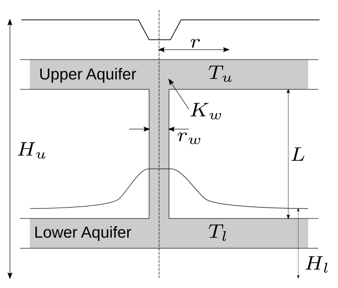
Figure 1: Illustration for the water flow through the borehole, adapted from Harper and Gupta (1983).
Inputs
For metamodeling applications (Morris et al., 1993; An and Owen, 2001; Kersaudy et al., 2015), the eight input variables of the borehole function are modeled as independent uniform random variables with specified ranges shown in the table below.
| No | Variable | Distribution | Parameters | Description |
|---|---|---|---|---|
| 1 | r_w | Uniform |
r_{w,\min} = 0.05, r_{w,\max} = 0.15 |
Radius of borehole [\text{m}] |
| 2 | r | Uniform |
r_{\min} = 100, r_{\max} = 50'000 |
Radius of influence [\text{m}] |
| 3 | T_u | Uniform |
T_{u,\min} = 63'070, T_{u,\max} = 115'600 |
Transmissivity of upper aquifer [\text{m}^2/\text{year}] |
| 4 | H_u | Uniform |
H_{u,\min} = 990, H_{u,\max} = 1'100 |
Potentiometric head of upper aquifer [\text{m}] |
| 5 | T_l | Uniform |
T_{l,\min} = 63.1, T_{l,\max} = 116 |
Transmissivity of lower aquifer [\text{m}^2/\text{year}] |
| 6 | H_l | Uniform |
H_{l,\min} = 700, H_{l,\max} = 820 |
Potentiometric head of lower aquifer [\text{m}] |
| 7 | L | Uniform |
L_{\min} = 1'120, L_{\max} = 1'680 |
Length of borehole [\text{m}] |
| 8 | K_w | Uniform |
K_{w,\min} = 9'885, K_{w,\max} = 12'045 |
Hydraulic conductivity of borehole [\text{m}/\text{year}] |
Other literature (e.g., Harper and Gupta, 1983) put alternative distributions on the variables r_w and r (while keeping the others the same) as shown in the table below.
| No | Variable | Distribution | Parameters | Description |
|---|---|---|---|---|
| 1 | r_w | Gaussian |
\mu_{r_w} = 0.10, \sigma^2_{r_w} = 0.0161812 |
Radius of borehole [\text{m}] |
| 2 | r | Lognormal |
\lambda_r = 7.71, \xi_r = 1.0056 |
Radius of influence [\text{m}] |
Resources
The vectorized implementation of the borehole function in MATLAB as well as the script file with the model and probabilistic inputs definitions for the function in UQLAB can be downloaded below:
uq_borehole.zip (3.1 KB)
The contents of the file are:
| Filename | Description |
|---|---|
uq_borehole.m |
vectorized implementation of the borehole function in MATLAB |
uq_Example_borehole.m |
definitions for the model and probabilistic inputs in UQLab |
LICENSE |
license for the function (BSD 3-Clause) |
References
- W. V. Harper and S. K. Gupta, “Sensitivity/Uncertainty Analysis of a Borehole Scenario Comparing Latin Hypercube Sampling and Deterministic Sensitivity Approaches”, Office of Nuclear Waste Isolation, Battelle Memorial Institute, Columbus, Ohio, BMI/ONWI-516, 1983. URL
- M. D. Morris, T. J. Mitchell, and D. Ylvisaker, “Bayesian design and analysis of computer experiments: Use of derivatives in surface prediction,” Technometrics, vol. 35, no. 3, pp. 243–255, 1993. DOI:10.1080/00401706.1993.10485320
- J. An and A. Owen, “Quasi-regression,” Journal of Complexity, vol. 17, pp. 588–607, 2001. DOI:10.1006/jcom.2001.0588
- P. Kersaudy, B. Sudret, N. Varsier, O. Picon, and J. Wiart, “A new surrogate modeling technique combining Kriging and polynomial chaos expansions – Application to uncertainty analysis in computational dosimetry,” Journal of Computational Physics, vol. 286, pp. 103–117, 2015. DOI:10.1016/j.jcp.2015.01.034