The two-dimensional heat diffusion model
The two-dimensional heat diffusion model has been used by Konakli and Sudret (2016) to test the performance of global sensitivity analysis using low-rank tensor approximations and Lüthen et al. (2021) to benchmark sparse polynomial chaos expansions. This approach allows for a detailed analysis of temperature distribution, focusing particularly on the average temperature in the region B = [-0.3, \,-0.2]^2 m.
Description
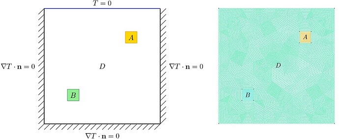
The heat diffusion model concerns two-dimensional thermal conduction within a square domain D = [-0.5, \,0.5]^2 with temperature field T(x), x\in D. The model is described by the partial differential equation:
It incorporates boundary conditions where T = 0 on the upper boundary and \nabla T \cdot \mathbf{n} = 0 on the left, lower, and right boundaries, where \mathbf{n} is the vector normal to the boundary.
The heat source Q\,1_A(x) is localized in A = [0.2, \,0.3]^2 m with Q = 2{,}000 W/m². The term 1_A(x) is the indicator function equal to 1 if x\in A and 0 otherwise.
The diffusion coefficient \kappa(x) is modeled as a lognormal random field with mean \mu_\kappa = 1 W/K \cdot m and standard deviation \sigma_\kappa = 0.3 W/K \cdot m, featuring an isotropic squared-exponential autocorrelation function with length scale \ell = 0.2 meters. For more details, see Konakli and Sudret (2016).
To discretize \kappa(x), the Expansion Optimal Linear Estimation (EOLE) method with 53 terms captures 99% of its variance. The solution to the heat diffusion problem is computed using an in-house finite element code. Inputs to the model consist of 53 independent standard normal random variables.
The response quantity of interest is the average temperature \bar{T} in the square domain B defined as:
Figure 1: Domain and boundary conditions (left) and finite-element mesh (right) of the two-dimensional heat diffusion model, adapted from Konakli and Sudret (2016).
Inputs
The two-dimensional heat diffusion model involves 53 independent Gaussian random variables:
| Variable | Description | Distribution | Statistics |
|---|---|---|---|
| X_1 - X_{53} | Input variable | Gaussian | \mu_{X_i} = 0, \sigma_{X_i} = 1 |
Open-access repository
The dataset used in this benchmark study is titled “Benchmark case datasets - Two-dimensional heat diffusion model” and is authored by Adéla Hlobilová, Stefano Marelli, and Bruno Sudret. It was published in 2024 and is available on Zenodo. The dataset can be accessed directly via the following DOI link: 10.5281/zenodo.12701147.
The experimental designs include datasets with 400, 800, 1200, 1600, and 2000 samples, each generated using optimized Latin Hypercube Sampling (LHS) with 1,000 iterations to improve the maximin criterion. Each dataset is replicated 20 times. The validation set contains 100,000 samples generated by Monte Carlo simulation. Each dataset contains samples and responses of the computational model.
For citation purposes, please use the following format:
Hlobilová, A., Marelli, S., and Sudret, B. (2024). Benchmark case datasets - Two-dimensional heat diffusion model. Zenodo. https://doi.org/10.5281/zenodo.12701147.
This project was supported by the Open Research Data Program of the ETH Board under Grant number EPFL SCR0902285.
References
- Konakli, K., Sudret, B. “Global sensitivity analysis using low-rank tensor approximations,” Reliability Engineering & System Safety, vol. 156, pp. 64–83, 2016. DOI:10.1016/j.ress.2016.07.012
- Lüthen, N., Marelli, S., Sudret, B. “Sparse Polynomial Chaos Expansions: Literature Survey and Benchmark,” SIAM/ASA Journal on Uncertainty Quantification, vol. 9, issue 2, pp. 593–649, 2021. DOI:10.1137/20M1315774
