Truss model
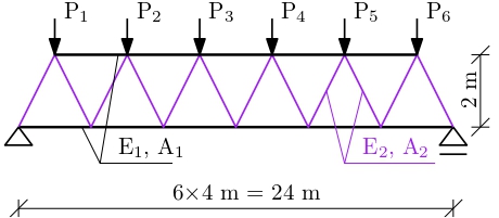
The 23-bar planar truss bridge (Blatman and Sudret, 2011) is a simply supported structure. Bars are categorized into two groups: the first group consists of 11 members, including the upper and lower chords, while the second group comprises 12 diagonals. The vertically oriented static loading is located in all six upper chord nodes. All truss bars are made from identical material.
Description
The response of the truss model is the mid-span deflection defined as:
where \mathbf{x} = \{E_1, E_2, A_1, A_2, P_1, ..., P_6 \} are independent input variables modeled by lognormal and Gumbel distributions.
Figure 1: The truss model, adapted from Dubourg (2011).
Inputs
For computer experiment purposes, the inputs E_1, E_2, A_1, A_2, P_1, ..., P_6 are modeled as ten independent random variables:
| No | Variable | Description | Distribution | Statistics |
|---|---|---|---|---|
| 1 | E_1 | Young’s modulus [Pa] | Lognormal | \mu_{E_1} = 2.10 \times 10^{11}, \sigma_{E_1} = 2.10 \times 10^{10} |
| 2 | E_2 | Young’s modulus [Pa] | Lognormal | \mu_{E_2} = 2.10 \times 10^{11}, \sigma_{E_2} = 2.10 \times 10^{10} |
| 3 | A_1 | Cross-sectional area [m²] | Lognormal | \mu_{A_1} = 2.0 \times 10^{-3}, \sigma_{A_1} = 2.0 \times 10^{-4} |
| 4 | A_2 | Cross-sectional area [m²] | Lognormal | \mu_{A_2} = 1.0 \times 10^{-3}, \sigma_{A_2} = 1.0 \times 10^{-4} |
| 5-10 | P_1 - P_6 | Load [N] | Gumbel | \mu_{P_1-P_6} = 5.0 \times 10^{4}, \sigma_{P_1-P_6} = 7.5 \times 10^{3} |
Resources
The vectorized implementation of the analytical solution of the mid-span deflection of the truss model in MATLAB, as well as the script file with the model and probabilistic inputs definitions for the function in UQLab, can be downloaded below:
uq_trussModel.zip (2.4 KB)
The contents of the file are:
| Filename | Description |
|---|---|
uq_trussModelAnalytical.m |
vectorized implementation of the truss model response in MATLAB |
uq_Example_truss.m |
definitions for the model and probabilistic inputs in UQLab |
LICENSE |
license for the function (BSD 3-Clause) |
Open-access repository
The dataset used in this benchmark study is titled “Benchmark case datasets - Truss model” and is authored by Adéla Hlobilová, Stefano Marelli, and Bruno Sudret. It was published in 2024 and is available on Zenodo. The dataset can be accessed directly via the following DOI link: 10.5281/zenodo.12699396.
The experimental designs include datasets with 100, 200, 300, 400, and 500 samples, each generated using optimized Latin Hypercube Sampling (LHS) with 1,000 iterations to improve the maximin criterion. Each dataset is replicated 20 times. The validation set contains 100,000 samples generated by Monte Carlo simulation. Each dataset contains samples and responses of the computational model.
For citation purposes, please use the following format:
Hlobilová, A., Marelli, S., and Sudret, B. (2024). Benchmark case datasets - Truss model. Zenodo. https://doi.org/10.5281/zenodo.12699396.
This project was supported by the Open Research Data Program of the ETH Board under Grant number EPFL SCR0902285.
References
- Blatman, G., Sudret, B. “Adaptive sparse polynomial chaos expansion based on least angle regression,” Journal of computational Physics, vol. 230, issue 6 pp.2345–2367, 2011. DOI:10.1016/j.jcp.2010.12.021
- Dubourg, V. “Adaptive surrogate models for reliability analysis and reliability-based design optimization”. Diss. Université Blaise Pascal-Clermont-Ferrand II, 2011. PDF file
- Lüthen, N., Marelli, S., Sudret, B. “Sparse Polynomial Chaos Expansions: Literature Survey and Benchmark,” SIAM/ASA Journal on Uncertainty Quantification, vol. 9, issue 2, pp. 593–649, 2021. DOI:10.1137/20M1315774
