Morris function
The Morris function has been used by Lamboni et al. (2012), Morris (1991) and Blatman and Sudret (2010) to test the performance of sensivity analyses.
Description
The performance function is defined as:
Different definitions of \omega_i and \beta ’s exist, we use the same as in Blatman and Sudret (2010):
- \omega_i = 2(X_i - \frac{1}{2}) for i \in \{1, 2, \ldots, 20\} and i \notin \{3, 5, 7\}
- \omega_i = 2\left(1.1 \frac{X_i}{X_i + 0.1} - \frac{1}{2}\right) for i \in \{3, 5, 7\}
- \beta_i = 20 for i \in \{1, 2, \ldots, 10\}
- \beta_{i,j} = -15 for i, j \in \{1, 2, \ldots, 6\} and i < j
- \beta_{i,j,l} = -10 for i, j, l \in \{1, 2, \ldots, 5\} and i < j < l
- \beta_{1,2,3,4} = 5
- \beta_i = (-1)^i for i \in \{11, 12, \ldots, 20\}
- \beta_{i,j} = (-1)^{i+j} for i \in \{1, 2, \ldots, 20\} and j \in \{7, 8, \ldots, 20\} and i < j
- \beta_{i,j,l} = 0 for i \in \{1, 2, \ldots, 20\}, j \in \{1, 2, \ldots, 20\}, l \in \{6, 7, \ldots, 20\} and i < j < l
- \beta_{i,j,l,s} = 0 for i \ne 1, j \ne 2, l \ne 3, s \ne 4
where:
- X_i: Random variables
- \omega_i: Functions of the random variables
- \beta: Coefficients
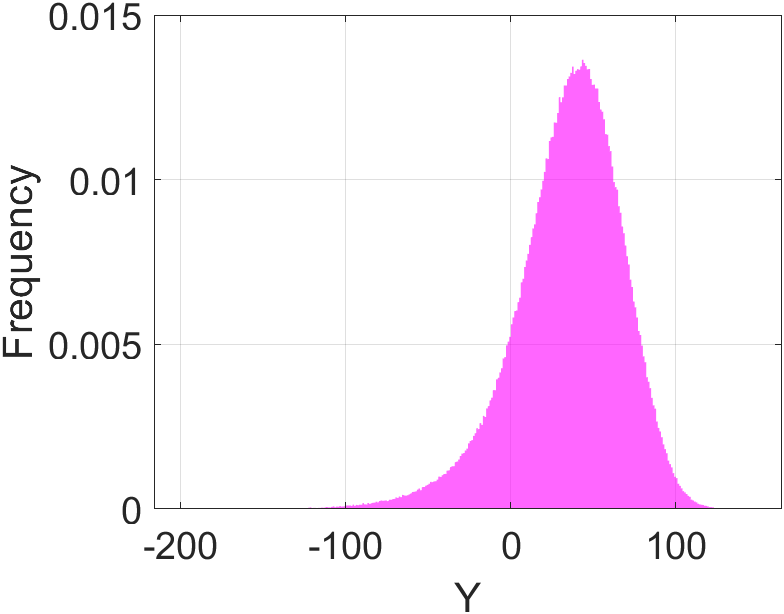
Figure 1: The histogram of the Morris function output when using uniform input distributions (see details below for the version by Blatman and Sudret (2010)) based on 10^6 sample points.
Inputs
The Morris function problem involves twenty independent random variables. Two specifications exist: one employs uniformly distributed random variables, while the other encompasses variables from various distributions. We utilize the specification from Blatman and Sudret (2010). For reference, we also present the alternative specification used in the literature by Lamboni (2012).
Version by Blatman and Sudret (2010):
| Variable | Description | Distribution | Parameters |
|---|---|---|---|
| X_1 - X_{20} | Input variable | Uniform | [0, \, 1] |
Version by Lamboni (2012):
| Variable | Description | Distribution | Parameters |
|---|---|---|---|
| X_1 | Input variable | Uniform | U(0,1) |
| X_2 | Input variable | Gaussian | N(0.5, \sqrt{0.1}) |
| X_3 | Input variable | Exponential | E(4) |
| X_4 | Input variable | Gumbel | G(0.2, 0.2) |
| X_5 | Input variable | Weibull | W(0.5, 2) |
| X_6 - X_{10} | Input variable | Uniform | U(0,1) |
| X_{11} | Input variable | Uniform | U(0,1) |
| X_{12} | Input variable | Gaussian | N(0.5, \sqrt{0.1}) |
| X_{13} | Input variable | Exponential | E(4) |
| X_{14} | Input variable | Gumbel | G(0.2, 0.2) |
| X_{15} | Input variable | Weibull | W(0.5, 2) |
| X_{16} - X_{20} | Input variable | Uniform | U(0,1) |
Resources
The vectorized implementation of the Morris function in MATLAB, as well as the script file with the model and probabilistic inputs definitions for the function in UQLab, can be downloaded below:
uq_Morris.zip (2.3 KB)
The contents of the file are:
| Filename | Description |
|---|---|
uq_morris.m |
vectorized implementation of the Morris function in MATLAB |
uq_Example_Morris.m |
definitions for the model and probabilistic inputs in UQLab |
LICENSE |
license for the function (BSD 3-Clause) |
Open-access repository
The dataset used in this benchmark study is titled “Benchmark case datasets - Morris function” and is authored by Adéla Hlobilová, Stefano Marelli, and Bruno Sudret. It was published in 2024 and is available on Zenodo. The dataset can be accessed directly via the following DOI link: 10.5281/zenodo.12700514.
The experimental designs include datasets with 400, 800, 1200, 1600, and 2000 samples, each generated using optimized Latin Hypercube Sampling (LHS) with 1,000 iterations to improve the maximin criterion. Each dataset is replicated 20 times. The validation set contains 100,000 samples generated by Monte Carlo simulation. Each dataset contains samples and responses of the computational model.
For citation purposes, please use the following format:
Hlobilová, A., Marelli, S., and Sudret, B. (2024). Benchmark case datasets - Morris function. Zenodo. https://doi.org/10.5281/zenodo.12700514.
This project was supported by the Open Research Data Program of the ETH Board under Grant number EPFL SCR0902285.
References
- Blatman, G., B. Sudret. “Efficient computation of global sensitivity indices using sparse polynomial chaos expansions,” Reliability Engineering & System Safety, vol. 95, issue 11, pp. 1216–-1229, 2010. DOI:10.1016/j.ress.2010.06.015
- Lamboni, M., B. Iooss, A.-L. Popelin, F. Gamboa. “Derivative-based global sensitivity measures: general links with Sobol’ indices and numerical tests,” Mathematics and Computers in Simulation, vol. 87, pp. 45–54, 2012. DOI:10.1016/j.matcom.2013.02.002
- Morris, M. “Factorial sampling plans for preliminary computational experiments,” Technometrics, vol. 33, no. 2, pp. 161-–174, 1991. DOI:10.2307/1269043
- Lüthen, N., Marelli, S., Sudret, B. “Sparse Polynomial Chaos Expansions: Literature Survey and Benchmark,” SIAM/ASA Journal on Uncertainty Quantification, vol. 9, issue 2, pp. 593–649, 2021. DOI:10.1137/20M1315774
