Beam problem:PCE surrogate model based calibration, how to give reasonable predictive posterior on multiple points?

Hi! Everyone. I am doing a classic simply-support-beam question.

image

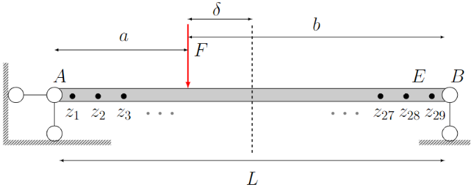
The input variables are Elastic modulus E and loading position \delta. I need to create my PCE surrogate model and doing Bayesian inference based on the 29 monitored data points along the beam.

This is my procedure:
Step 1: Refer to PCE - Calculation strategies | Examples | UQLab, create my PCE
Step 2: Bayesian inversion - MAP estimation | Examples | UQLab, doing my Bayesian inference to get E and \delta

The code works well and it converges very well for the simple beam problem. But I have a question for the result I get.

image
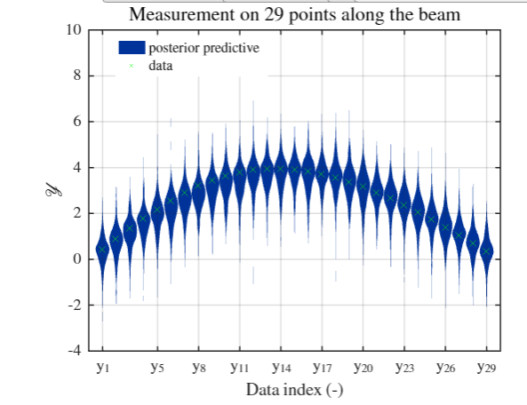
(please ignore the big range of predictive distribution. It should be very small. I make it very large on purpose to make it obvious)

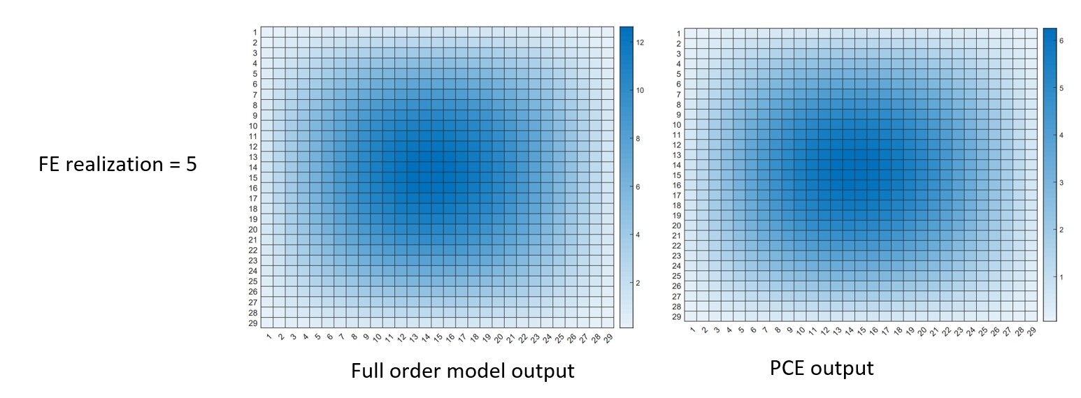
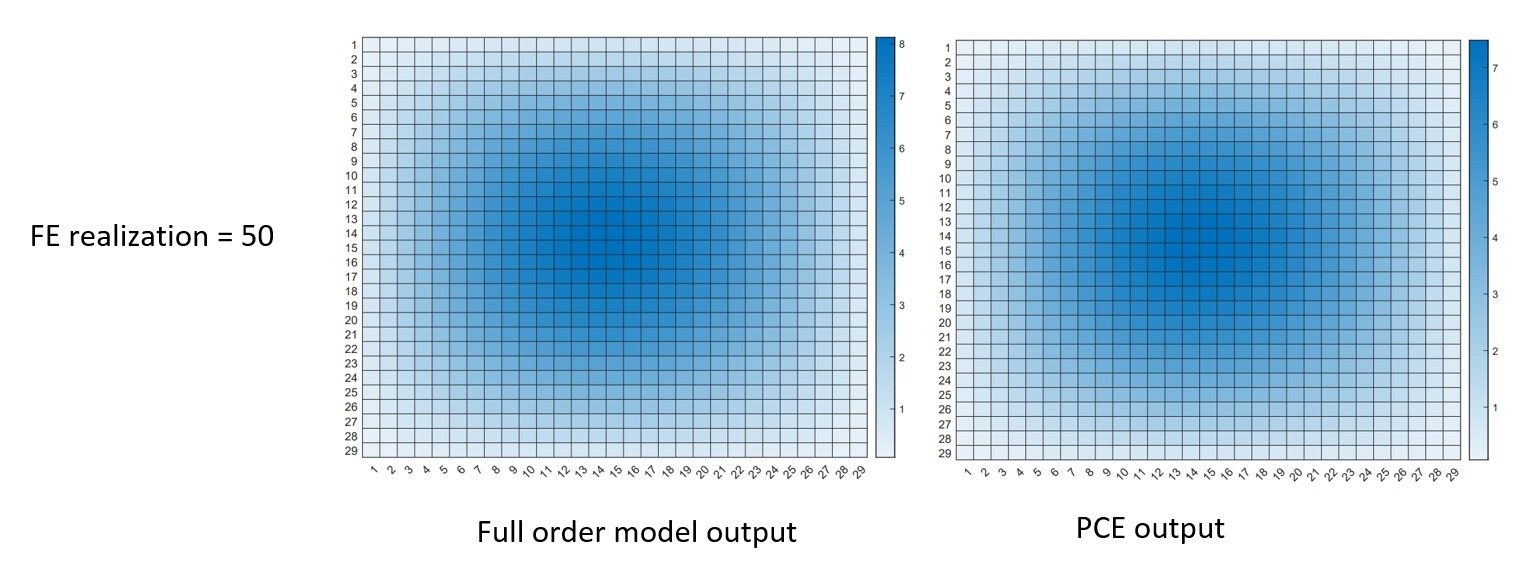
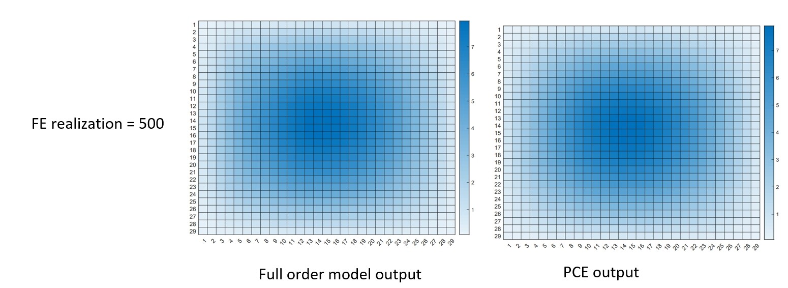
Anyway, in the PCE that I create, based on the 29 output points along the beam, I get a 29 independent sub-PCE model in the PCE model, right? Because it mentioned “UQLAB performs an independent PCE for each output component on the shared experimental design” in the UQLab - Polynomial chaos expansions (PCE) user manuals.

So, my question is : Since the 29 sub-PCE (though combined in one PCE structure) for each point along the beam is independent, how can we make reasonable predictive posterior? for example, as shown the red line in the picture, it is reasonable in probabilistic theory but unrealistic in life. Or in another way, can we consider the relationship between 29 sub-PCEs ? or how we avoid this unrealistic predictive outcome?

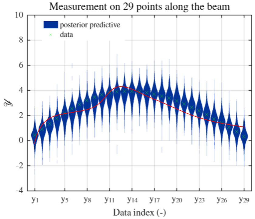
I personally think the problem comes from the fact "every PCE model is independent ", they each have no connections. Can someone help me this question? thanks in advance!!!
code is attached
PCE_multiple.zip (265.8 KB)

1 Like

Dear @ny123

Thanks for your question. This is very relevant, but there is some misunderstanding in the way PCEs are constructed and used in the Bayesian framework.

When the manual says “every PCE is built independently”, it simply means that the input data \mathcal{X} and the output \mathcal{Y}_i is used separately for each output i (in other words, there is a loop on the components of the output for the construction). However, from the physics, the output samples (\mathcal{Y}_i, \mathcal{Y}_j) are correlated (even strongly correlated if you look at two neighbor points). The resulting PCEs will show the same correlation. In fact, the covariance between two PCE outputs can be computed analytically. If:

Y_i = \sum_{\alpha \in \mathcal{A}} a_{\alpha} \, \Psi_{\alpha}(\mathbf{x}) \quad ; \quad Y_j = \sum_{\alpha \in \mathcal{A}} b_{\alpha} \, \Psi_{\alpha}(\mathbf{x})

then the covariance read:

\text{Cov}\left[{Y_i, Y_j}\right] = \sum_{\alpha \in \mathcal{A} \backslash 0} a_{\alpha}b_{\alpha}

and their linear correlation coefficient is obtained by normalizing with their respective variances. As a conclusion, “built independently” does not mean that the resulting PCEs are statistically independent.

Now, if we come back to the Bayesian inversion problem, you should pay attention to two points:

  • the discrepancy model between model prediction and measurement data: it could be set independent for the 29 measurement points, but it could also be a joint Gaussian vector with nondiagonal covariance matrix.
    If this discrepancy only represents measurement error (typically, very small), then it makes sense that the sensors are independent. If, however, it also represents a systematic model error (maybe not relevant for your example here, but rather common in realistic applications), then typically a correlation structure of the mismatch should be assumed and fitted altogether within the Bayesian inversion [1,2].
  • This possibly correlated Gaussian mismatch model should be properly propagated when you sample the predictive distributions.

Also note that the posterior distributions of the X’s are often correlated, which has to be taken into account when sampling the predictive distributions of the Y’s.

I hope it clarifies your problem! Best regards

Bruno

References
[1] Wagner, P.-R., Fahrni, R., Klippel, M., Frangi, A., Sudret, B., 2020. Bayesian calibration and sensitivity analysis of heat transfer models for fire insulation panels. Engineering Structures 205.
[2] Wagner, P. R., 2021. Stochastic spectral embedding in forward and inverse uncertainty quantification, PhD thesis, ETH Zurich.

1 Like

Hi @ny123 and @bsudret, some more discussion on the roles of modelling error from PCE in the context of Bayesian inversion and high dimensional output models, you can have a look at: Bayesian tomography with prior-knowledge-based parametrization and surrogate modelling | Geophysical Journal International | Oxford Academic

Cheers,
Stefano

Dear @bsudret ,

Thanks very much for your detailed explanations for PCE constructions and how it works in the Bayesian inference. And I think your answer totally solved my misunderstandings for the PCE covariance.

As you said, “the output samples (\mathcal{Y}_i, \mathcal{Y}_j) are correlated and the covariance can be computed analytically”, it is true and I compared with the FE output covariance and PCE output covariance.
With more and more realizations, the covariances becomes more and more similar and finally identical.


And also, your suggestions on the Bayesian inference are very helpful and I have read Wagner’s paper you recommended. Those are very helpful and good references to PCA-PCE models. I will deal with the discrepancy model covariance (non-diagonal) carefully in the bayesian inversion.

Best,
ningxin

Dear @ste ,

Thanks for recommending this paper and this is a very good implementation for the high dimension surrogating problem. It seems in this paper that the covariance matrix for the modelling error can be handled in a relative smooth way. Thanks for your paper. I will read it very carefully and I think it will give me a lot of help!

Best
ningxin