Dear felix,
I think that there are some UQLab featrues that may help you out of the box, but I am not sure if they
are sufficient for you.
One remark in advance.:
It holds in both for your files that your settings for Solver are not copied to BayesOpts.Solver at the end (see UQLab Manual 3.1.4) such that all your settings are ignored at the end and the default values are used. This can be seen for example in the trace plots above ending after 300 steps.
- If you want, for example, compare the prior and posterior density for E1, you can use the commands
% Using the default value of  BayesOpts.Solver.MCMC.Steps being 300, the
% default value of  BayesOpst.Solver.MCMC.NChains being 100  for the default
% AIES-MCMC scheme and the default value of 0.5 for burnIn there are  151
% steps in  myBayesianAnalysis_surrogateModel.Results.PostProc.PostSample
% each with 100 values, i.e. there are 15100 samples values for the posterior
% densithy that are provided as input data to the plot function. To get plots
% that can be compared, we need a similar number  samples for the prior
% that are generated by the following call of uq_postProcessInversion
% Attention: In the following line there was an incorrect 5000 in the original version of this post
 uq_postProcessInversion(myBayesianAnalysis_surrogateModel,'prior',15100);
uq_display(myBayesianAnalysis_surrogateModel,'scatterplot',1)
leading to two figures similar to
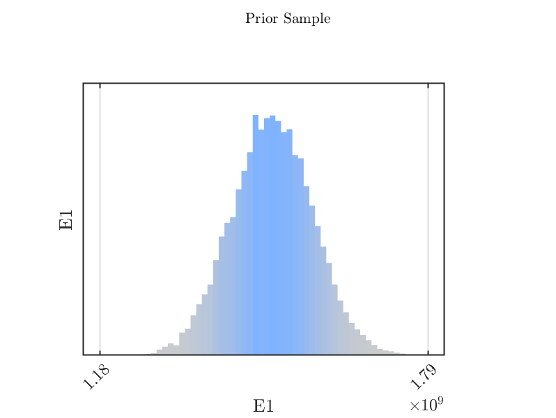
and
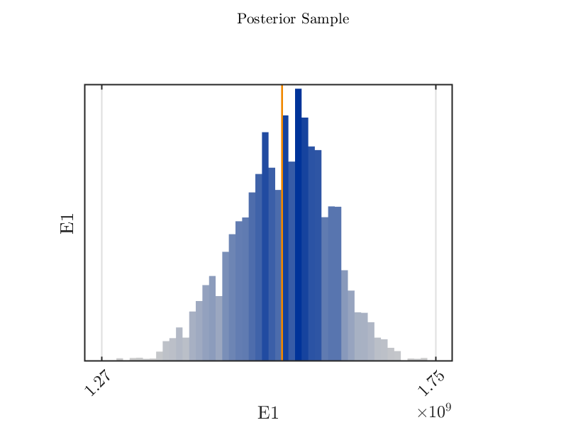 .
.
-
In the original UQLab 1.4.0 version of
uq_display_uq_inversion.mthe limits for the plots for the posterior density are determined from the limits for the plots for prior density, see my topic to this behavior. Hence, you can use these plots to compare prior and posterior densities. -
In view of the plots above your may need more samples for both densities to get nice plots for both densities.
-
I would not be surprised if there are MATLAB methods to combine the two figures created by
uq_displayvia callinguq_display_uq_inversionsomehow after you managed to get the handles for them but this is beyond my MATLAB skill. -
An other way to get one plot with prior and posterior density is (after following step 3) to copy the contents of
myBayesianAnalysis_surrogateModel.Results.PostProc.PriorSampleand of
myBayesianAnalysis_surrogateModel.Results.PostProc.PostSample, following the instructions by Paul-Remo to rearrange the copy of....PostSampeand use afterwards the MATLAB commandhistogramto generate a plot with histograms for both data sets.
Greetings
Olaf