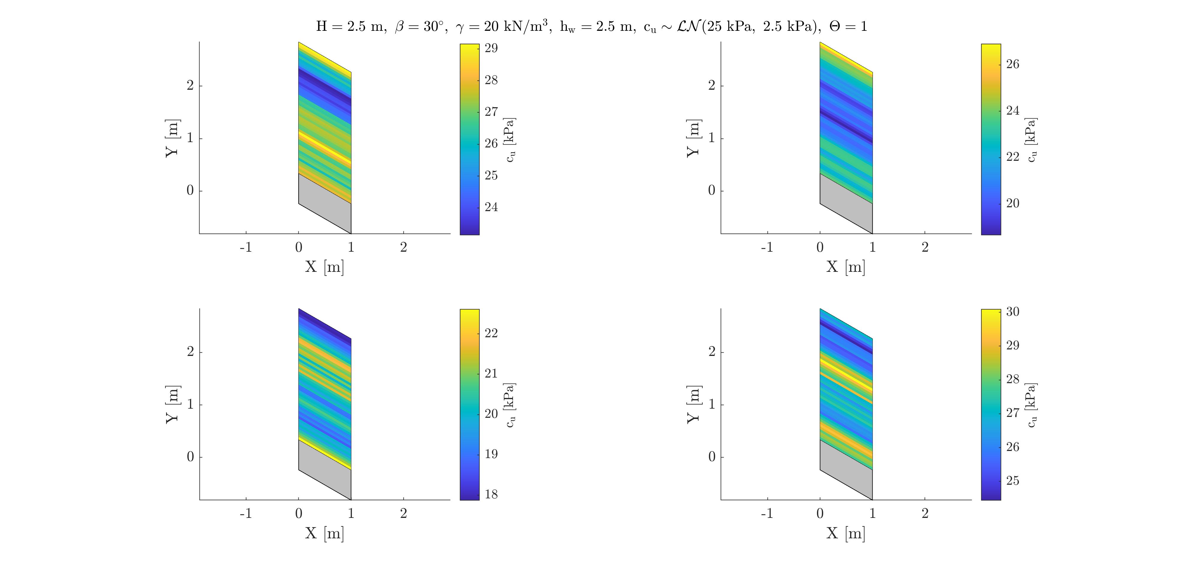
I wrote in Matlab a code which generates 1D unconditional random fields following section 2.1.2 of “Application of conditional random fields and sparse polynomial chaos expansion to geotechnical problems” and it seems to work well. For example, I use it to model spatial variability of cohesion dependent on the depth in the soil layer. Attached a picture with 4 realizations of a depth dependent soil cohesion created with my code. The question is, how to generate random fields for 2D spatial variability? What I would like to have is for example soil cohesion which is dependent on the position (x,y) and not only on the depth y. More precisely, I don’t understand which size the covariance matrix is going to have. In 1D spatial variability, if my domain is discretized by 10 points, then my covariance matrix is going to be 10X10, but what if my domain is discretized by 10 point in x and y direction?
There is little change between generating 1D or 2D random fields. To apply the EOLE method, you start with a grid of support points: instead of having n points on a line with a single coordinate z, you need to define a 2D grid of n_x \times n_z points. Then you need a 2D correlation function. In geotechnics we often use the product of two functions of x and z, yet with different correlation lengths. For instance, with a square-exponential function: \rho(\boldsymbol{x}_1,\boldsymbol{x}_2) = \exp\left[ -(\frac{x_1 -x_2}{\ell_x})^2 - (\frac{z_1 -z_2}{\ell_z})^2\right] .
Then you compute the correlation matrix between the points of your grid (which is now a matrix of size n_x \times n_z) and the rest follows as in the 1D case.
What is important is to select a proper grid step size (distances \Delta_x and \Delta_z between neighbour points) in coherence with i) the type of correlation function and ii) the correlation lengths \ell_x and \ell_z. All this is discussed in all details in the State-of-the-art report on stochastic finite element and reliability analysis. Also, the truncation of the series expansion should be carried out carefully based on the explained variance, see above report.
Well, it was my first work in the field of UQ and reliability back in … 2000 ( ), so I would not claim it is “state-of-the-art” any more, especially on polynomial chaos expansions. However, the part on discretizing random fields is still OK.
 ), so I would not claim it is “state-of-the-art” any more, especially on polynomial chaos expansions. However, the part on discretizing random fields is still OK.