Bayesian inference with multiple forward model with different numbers of provided measurements but with one common discrepancy model and parameter?

Dear Paul-Remo,

Thanks for you suggestion. I am sorry, but it seems to me that using your idea creates problems at least due to a consistence check in uq_initialize_uq_inversion.m. In view of the lines 171 - 178 in this file it seems to be requested that every output index is only used once for each model, at least within in one data group. Do you think I could try to deactivate this consistence check even if deactivating checks is generally a bad idea, since maybe the code evaluated n the following needs that this consistency is satisfied?

I have tried to apply your suggestion to the file SCR_BI_to_25_Sugest.m (2.3 KB) derived from the example in the UQLab User Manual on Bayesian Inference, and got the error message:

The supplied MOMap does not uniquely address every model output

Error in uq_initialize_uq_inversion (line 176)
error(‘The supplied MOMap does not uniquely address every model output’)

Error in SCR_BI_to_25_Sugest (line 68)
myBayesianAnalysis = uq_createAnalysis(BayesOpts);

Dear Olaf

Thanks for the file - my bad. I previously checked your problem on the next version of UQLab that is currently under development instead of the currently live version.

Yes, you can safely comment out the check in uq_initialize_uq_inversion lines 175-177.

Let me know how it goes!

Dear Paul-Remo,

thanks for your answer. I am still on my way of understanding and testing
your suggestion, but I have already a small remark and a big one:

1.) Since consistency checks have quite often saved my day by pointing out
that I made some typo etc. I would prefer to keep the consistency check
in general, but to allow some override by adding a list in data.MOMapNotUnique
of those models to point out that I really want to reuse at least one of
outputs of the model. Hence, I replaced in uq_initialize_uq_inversion
the lines 175-177 by

 if length(unique(CurrModelOMap)) ~= length(CurrModelOMap)
       if ~isfield(Opt.Value(1),'MOMapNotUnique')
            fprintf('\n Problem with model \%g\n',ii);
            error('The supplied MOMap does not uniquely address every model output and no exception list in MOMapNotUnique is provided')
        elseif ~ismember(ii,Opt.Value(1).MOMapNotUnique)
            fprintf('\n Problem with model \%g:\n',ii);
            error('The supplied MOMap does not uniquely address one model output and the model is not listed in the exception list in MOMapNotUnique')
        \% else case would correspond to the situation that the supplied
        \% MOMap does not uniquely address every model output but that is
        \% no error and therefroe announced by inserting the model
        \% number in the exception list in MOMapNotUnique
        \% BUT, one may have to add a further check to ensure that 
        \% that no output does appear in several data groups to ensure 
        \% the the outout has one unique discrepancy assigned to it,        
        end
    elseif  isfield(Opt.Value(1),'MOMapNotUnique')  && ismember(ii,Opt.Value(1).MOMapNotUnique)
        fprintf('\n Problem with model \%g:\n',ii);
        error('The supplied MOMap does uniquely address all outputs for this model but the model is listed in MOMapNotUnique')
    end
  1. To understand the results of my tests I needed to learn more on the components of

myBayesianAnalysis.Results.PostProc

that are not discussed in the manual. Hence, I examined the code in uq_postProcessInversion.m and realized that deactivating the consistency check may have side effects that can be quite surprising, at least according to my humble opinion:

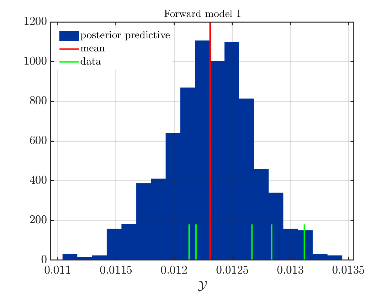
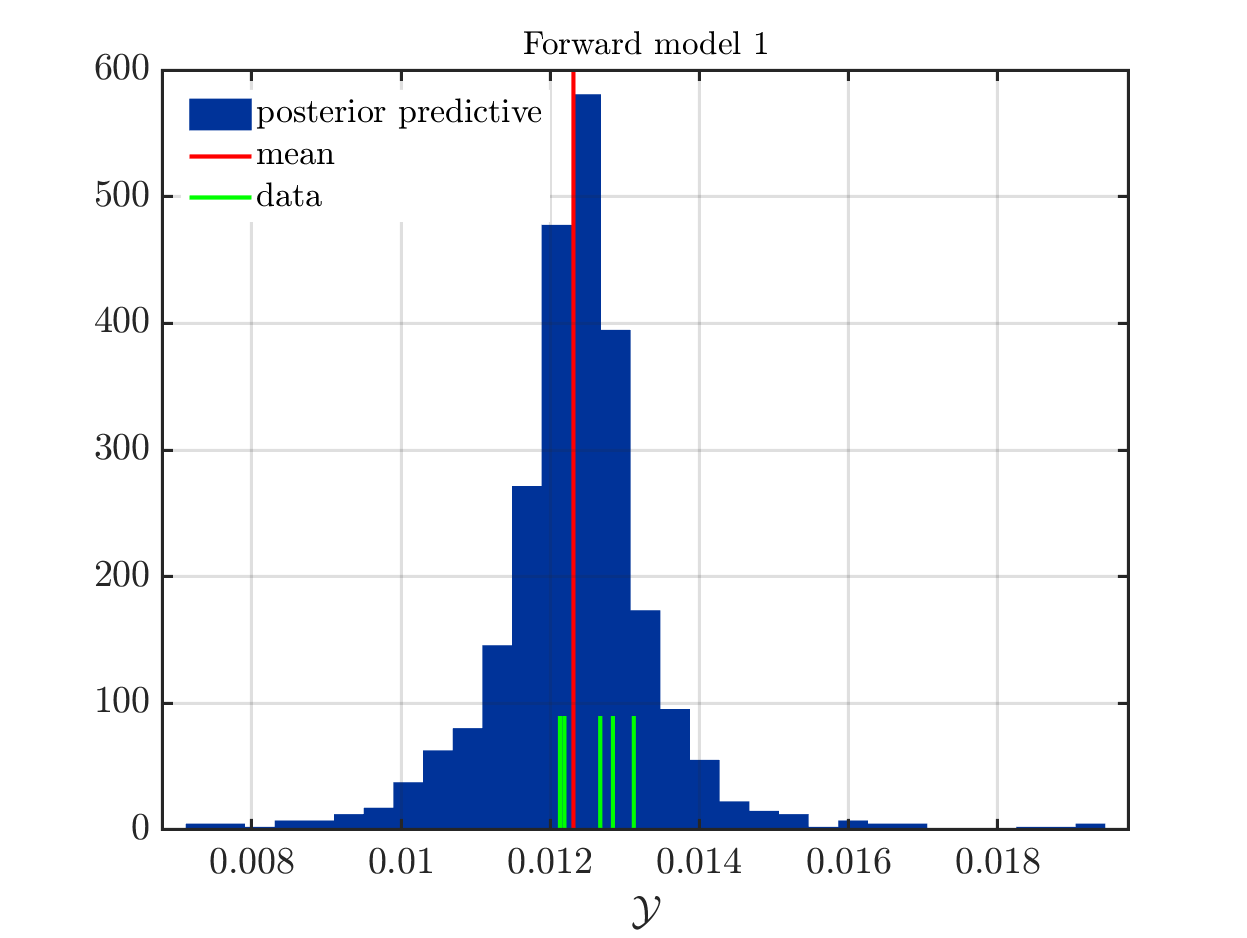
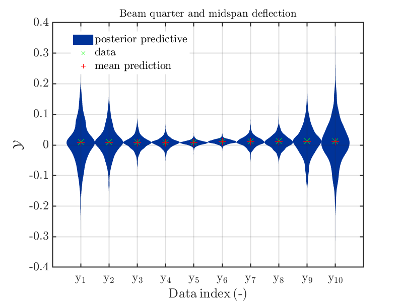
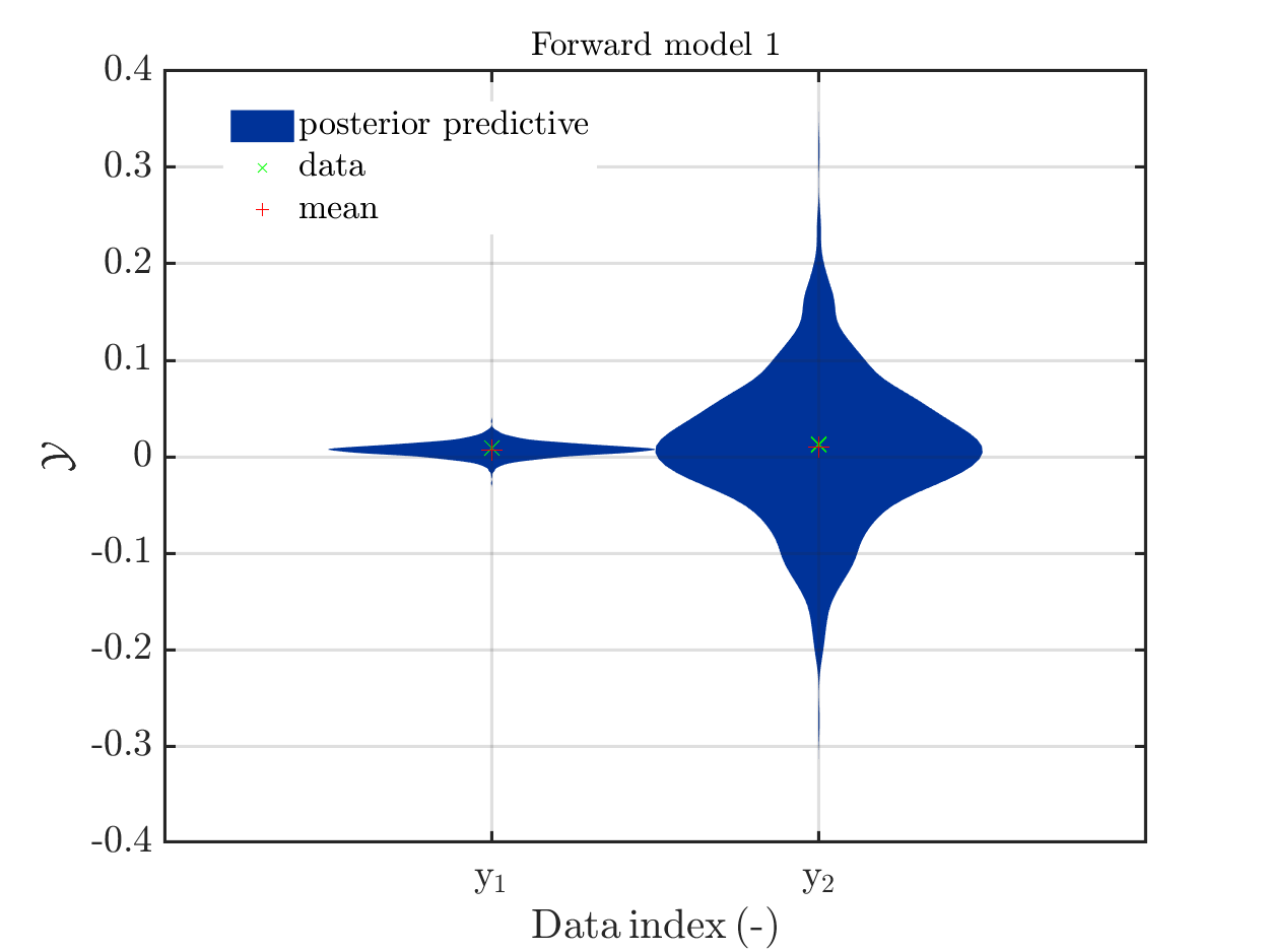
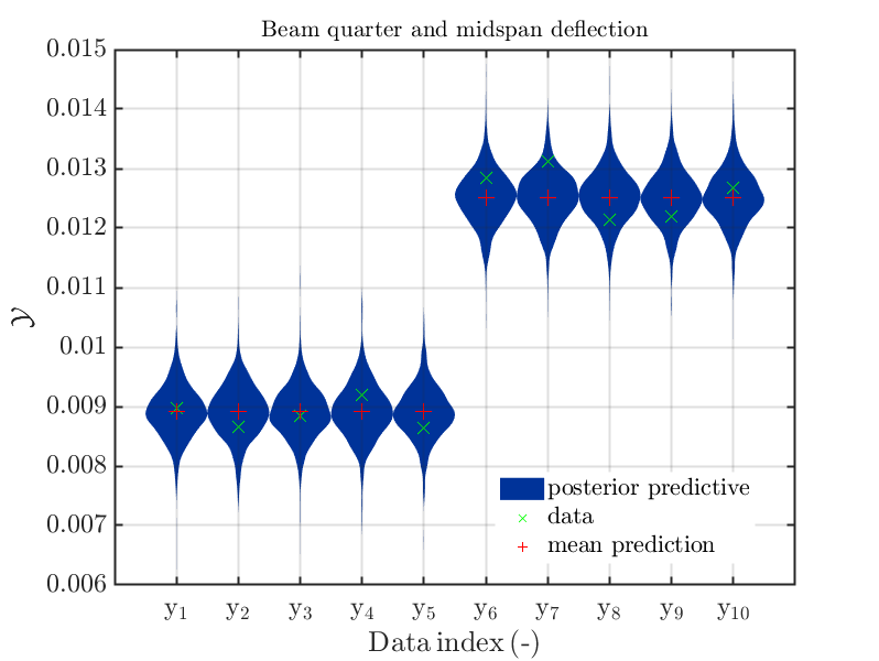
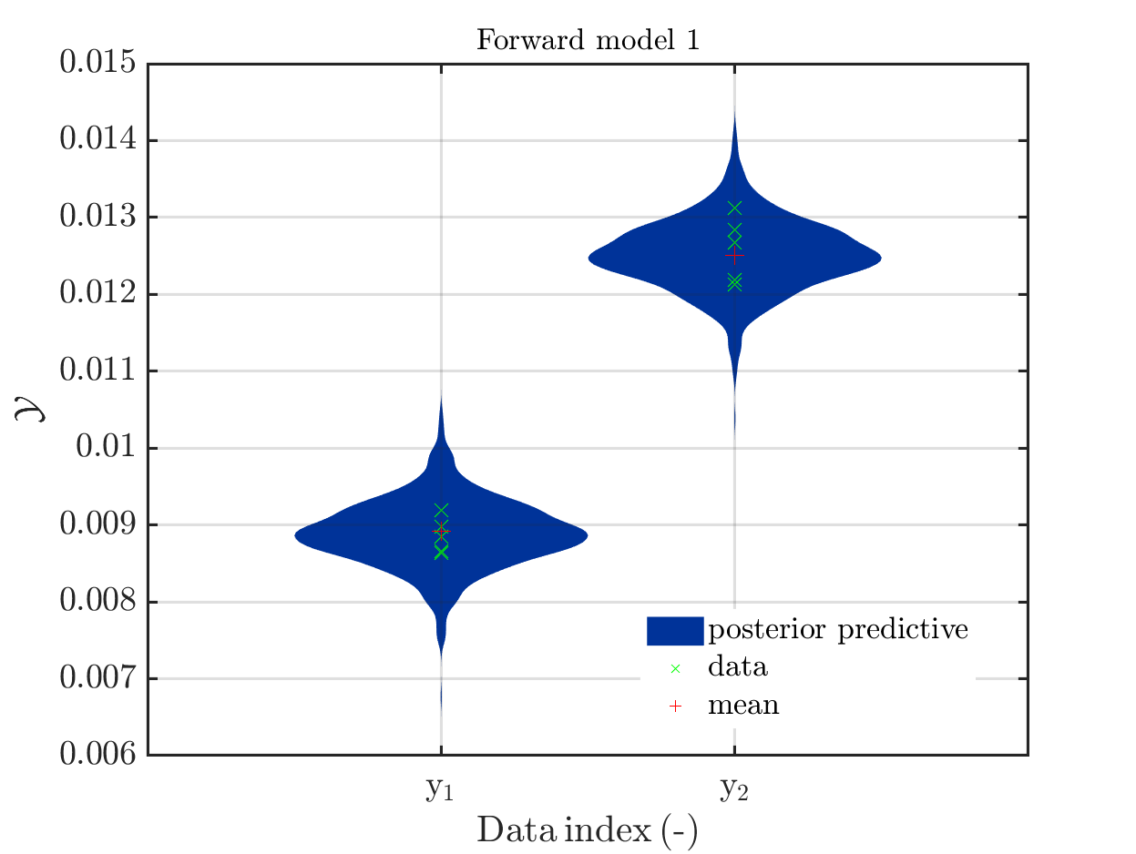
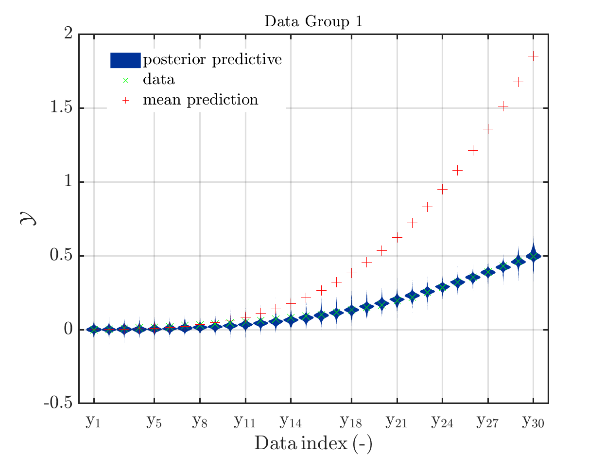
If one is using the same model output in two discrepancy data groups, one can change the resulting posterior predictive distributions plot by exchanging the groups, see SCR_DataGroup.m (2.5 KB) and SCR_DataGroupExc.m (2.6 KB) leading to the posterior predictive distributions plots in


and in

, respectively.

This is a emulation of the situation that a UQLab-user has two sets of measurements for the same model, one with many measurements and some discrepancy and a second one with less measurements but also a smaller discrepancy.
Using two discrepancy data groups with two different UQLab models, both using the same function, the UQLab-user can identity the model parameter and can get two separate scatter plots. To get one combined scatter plot the UQLab-user may try to use the same UQLab model in both discrepancy data groups since she/he exepects that the created posterior predictive sample points used for the scatter plot, i.e.the contents of

myBayesianAnalysis.Results.PostProc.PostPred.model(mm).postPredRuns

are somehow randomly choosen from all predictive sample values computed in both (all) data groups.
(It holds for

myBayesianAnalysis.Results.PostProc.PostPred.model(mm).data

that the data sets provided in the different discrepancy data groups are connected
in one data set.)

But, this is not the case: Considering line the loop in the lines 520 to 576 in uq_postProcessInversion.m one realizes that for every model mm and every output number modelOutputNr it holds that

model(mm).postPredRuns(:,modeCompNr)

is equal to the predictive sample computed in the last discrepancy data groups containing the output modelOutputNr of model mm.

I think this is a problem one has to be aware of and may require to either disallow to use one model output in several discrepancy data groups or to change the loop discussed above to do same sampling between the different predictive sample values for the considered model output.
But, before chancing the loop one would need to fix a well defined way to choose predictive sample values for a model output if there are several data groups each one generating several predictive sample values, such that the loop in lines 563 - 575 starts with a field postPredRunsCurr, such for each index kk it holds that postPredRunsCurr(kk,: ) contains several several predictive sample values for the considered model output.

But, this is no direct problem for me since currently I plan to use only one discrepancy data group and will now continue my testing and will start to connect my problem to UQLab in the near future.

Best regards
Olaf

1 Like

Dear Olaf

You are right - the computation of the posterior predictive distribution fails when the check for the uniqueness of the MOMap is disabled in the initialization. In fact, the theory section of the current Bayesian manual is missing a proper introduction of data groups and associated posterior predictive distribution computation. I attach below a new subsection that will be included in the next version of the Bayesian module containing such an introduction.

1.2.4 Multiple data groups
In practice it occurs frequently that the measurements \mathcal{Y} stem from various measurement devices or experimental conditions with different discrepancy properties. In these cases, it is necessary to arrange the elements of \mathcal{Y} in disjoint data groups and define different likelihood functions for each data group.

Denoting the g-th data group by \mathcal{G}^{(g)} = \{\mathbf{y}_i\}_{i\in\boldsymbol{\mathsf{u}}}, where \boldsymbol{\mathsf{u}}\subseteq\{1,\cdots,N\}, the full data set can be combined by

\mathcal{Y} = \bigcup_{g=1}^{N_{\mathrm{gr}}}\mathcal{G}^{(g)}.

Each of the N_{\mathrm{gr}} data groups contains measurements collected with the same instruments under similar measurement conditions. With this, it is clear that each data group requires a different likelihood function \mathcal{L}^{(g)} describing the experimental conditions that led to measuring \mathcal{G}^{(g)}. Possible choices for \mathcal{L}^{(g)} are presented in Section 1.2.2 and Section 1.2.3.
Under the assumption of independence between the N_{\mathrm{gr}} measurement conditions, the full likelihood function can then be written as

\mathcal{L}(\mathbf{x}_{\mathcal{M}}, \, \mathbf{x}_{\mathcal{\varepsilon}};\mathcal{Y}) = \prod_{g=1}^{N_{\mathrm{gr}}}\mathcal{L}^{(g)}(\mathbf{x}_{\mathcal{M}}, \mathbf{x}_{\mathcal{\varepsilon}}^{(g)};\mathcal{G}^{(g)}),

where \mathbf{x}_{\mathcal{\varepsilon}}^{(g)} are the parameters of the g-th discrepancy group.

With this, it is natural to define predictive distributions for each data group individually through

\pi''^{(g)}_{\mathrm{pred}}(\mathbf{g}\vert\mathcal{Y}) = \int_{\mathcal{D}_{\mathbf{X}}}\mathcal{L}^{(g)}(\mathbf{x};\mathbf{g})\pi(\mathbf{x}\vert\mathcal{Y})\,\mathrm{d}\mathbf{x}

where \mathbf{g} is a variable collecting only the outputs addressed in the g-th data group.

In the current version of the Bayesian module (1.3.0), every model output can only be compared to one data point (and possible multiple measurements thereof). The predictive distributions are therefore expressed for each forward model independently.

When the restriction of uniqueness is lifted, however, this is no longer possible because the same model output might be compared to measurements of different data groups. To properly express the predictive distributions, the original formulation will be used in the next version of UQLab. The predictive distributions will, therefore, be computed and plotted for each data group separately. This distribution then captures the uncertainty we expect in measurements made with the g-th measurement device.

To get back to your specific problem, I attach three functions from the upcoming next version of the Bayesian module that you can use to overwrite the existing functions of the same name. You should then be able to run your analysis with non-unique MOMap entries.

uq_display_uq_inversion.m (19.9 KB)
uq_initialize_uq_inversion.m (30.9 KB)
uq_postProcessInversion.m (19.4 KB)

I hope this clarifies your questions - let me know if it does not and I greatly appreciate your in-depth review of the module.

1 Like

Dear Paul-Remo,

thank your for your answer, especially the pre-version of the new part in the documentation and new versions of the module files. I will start to test, after informing you about a suggestion for a fix for a well-hidden bug that is also active (and hidden) in your new version of uq_initialize_uq_inversion.m

I suggest to replace the in the lines 89-90 in uq_initialize_uq_inversion.m the name of the variable “ForwardModel” by an other one, for example “ForwardModelFromOptValue” to avoid that in line 415 the variable “ForwardModel” on the left-hand side is accidentally already defined as up_model.
This has produced some quite strange error message when I used
BayesOpts.ForwardModel = myForwardModel with myForwardModel being a single UQLab-Model instead of relying, as most other users do, on the default behavior of UQ-Lab to use the last created MODEL object (in this case also myForwardModel) as the forward model if uq_creasteAnalysis is called.

When I evaluated SCR_BI_to_233_test.m (1.5 KB) I got the
error message:

Unrecognized property ‘Model’ for class ‘uq_model’.

Error in uq_initialize_uq_inversion (line 415)
ForwardModel(ii).Model = uq_createModel(ModelOpt,‘-private’);

Error in SCR_BI_to_233_test (line 48)
myBayesianAnalysis = uq_createAnalysis(BayesOpts);

And I must admit that I need some debug runs to realize that the problem was not
in the evaluation of uq_createModel(ModelOpt,’-private’).

Best regards
Olaf

1 Like

Dear Olaf

Thank you very much! This is a great catch - this bug will be fixed in the next version.

Dear Paul-Remo,

I have again used UQLab in a way not planed by the developers, such that I found some further problems that I have now formulated within the feature request uq_postProcessInversion: Extension of docmentation to deal with multiple calls of this function, code corrections and extension .

I would like to point out that using your new files I get from you , uq_Example_Inversion_04_PredPrey.m generates the following plot for the second mode:


and I wanted to get rid of the samples for the priori predictive distribution to
get a plot like this .

Using your version of uq_postProcessInversion.m it holds that the call

uq_postProcessInversion(myBayesianAnalysis,…
‘badChains’, badChainsIndex,…
‘priorPredictive’, 0, …
‘posteriorPredictive’, 1000);

generated the error

Index exceeds matrix dimensions.

Error in uq_postProcessInversion (line 447)
   priorRunsCurr(:,MIndex) = model(mm).priorRuns(:,OMapCurr);

i.e. only the line number is changing with respect to the normal version of
uq_postProcessInversion.

Thanks again for your files.

Greetings
Olaf

Dear Olaf

Thanks for pointing this out - what you found is a parser issue in the initialization of uq_postProcessInversion, where the drawing of prior, prior predictive and posterior predictive samples was not deactivated when the user requested 0 samples.

This issue will be fixed in the upcoming version of the inversion module.

Dear Paul-Remo,

I have now two further issues:

1.) During testing, I considered the situation of two data groups, the first one with a material with vectorial output and the second one with a scalar output by combining Sections 2.5 and 2.3 in the manual.

The code seemed to work as long as no samples for the prior predictive distribution the are computed. But after samples for the prior predictive distribution were derived by corresponding call of uq_postProcessInversion the call of uq_display see SCR_BI_to_25_23.m (2.9 KB)
creates the following error message during the plot for the second data group:

Error using histc
Edge vector must be monotonically non-decreasing.

Error in hist (line 126)
    nn = histc(y,edgesc,1);

Error in uq_histogram (line 97)
    [hY,hX] = hist(Y,X);  % X are the centers of the histogram elements

Error in uq_display_uq_inversion>plotSinglePred (line 453)
        postPlot = uq_histogram(postRuns, xData, 'FaceColor', postColor);

Error in uq_display_uq_inversion (line 335)
                plotSinglePred(Sample(ii),DataCurr,plotType,pointEstimatePred)

Error in uq_module/Display

Error in uq_display (line 4)

Using the old files, I get the same result, just with
uq_display_uq_inversion>plotSinglePred (line 436)
Error in uq_display_uq_inversion (line 324)

2)
I fear I have a problem with your new kind of plots generatred if one component of one material apperas several times in MOMap, i.e. think I need in addition also
the old kind of plots (maybe with some modifications). I do not now, if I should formulate this as a further feature request, since the question of the possible plot
in the situation that the contents of MOMap are not unique may be of more general interest. What do you think?

Greetings
Olaf

Hi Olaf

Regarding your first question: You have uncovered a bug in the uq_display_uq_inversion function.

First of all, a hold on is missing after

priorPlot = uq_histogram(priorRuns, 'Facecolor', priorColor);
hold on

secondly, and this is quite embarrassing :roll_eyes:, the first two arguments of the second uq_histogram function are switched. They should be

postPlot = uq_histogram(xData, postRuns, 'FaceColor', postColor);

I attach the corrected uq_display_uq_inversion function for your convenience.
uq_display_uq_inversion.m (19.9 KB)

Regarding your second question, I am not sure I understand what you mean. Are you referring to the possibility to plot predictive distributions for each model as opposed to for each discrepancy group?

Dear Paul-Remo,

thanks for dealing with this pug and for your new files.

In my second question, I am referring to the possibility to plot (within one discrepancy group) predictive distributions for each output component for each model as opposed to for each component in the data vector aka for each component in the NOMap vector, since my data vector will have more then 450 components.

To explain this in more details, lets consider the example as in Section 2.3 of the manual and its reformulation according do your suggestion in your initial reply in this discussion.

Allowing different discrepancies for the components and using quite different prior densities for them, see Multi_10Dis.m (3.8 KB), your new plot function produces Multi_10Dis-newUQLab
containing 10 plots, while using the normal UQLab version (with some dealing with
nonunique entries in MOMap) generates the figure
Multi_10Dis-oldUQLab
showing only plot No. 5 (with the data marks from plots 1-5) and plot No. 10 (with the data marks from plots 6-10) from the figure before. Hence, we see that the figure generated by the normal UQLab are incomplete and that the figure generated by your new files is complete and allows to directly compare the different posterior predictive distributions for the components.

But, if one is considering a joined discrepancy for all components the differences are lees important: Using Multi_oneDis.m (2.3 KB) and your new UQLab-files, one gets: Multi_oneDis-newUQLab
Using the old UQLab-files (with my update), one gets the figure
Multi_oneDis-oldUQLab
showing again only the 5th and the 10th distribution presented in the plot before, incorporating also the corresponding data marks.But, here this is not a problem to show only these two plots, since the plots 1-5 are almost identical, and also the plots 6-10 are almost identical.

This corresponds somehow to the situation in my application, but there is an important difference due to the amount of my data. Using your new data extraction and plot routines, I would get a figure starting with two groups with 29 plots followed by one group with 28 plots, one group with 27 plots, …, one group with 2 plots and finally one group with one plot, i.e. I would have 464 plots overall in one figure. I fear that one what not be able to see much in these figure since the individual plots would become very, very small. Using the old UQLab functions I would get a figure with 30 plots, each one involving the corresponding data points.

Hence, I would be grateful, if there would be a way to get also the old kind of plots without reactivating the old UQLab version, at least for discrepancy groups with only one joined discrepancy density.
Maybe one could improve these plots by using as title for the figure the name of the model, and by changing the description off the horizontal axis, i.e. by replacing ‘data index’, ‘y_1’ and ‘y_2’ by something like ‘output index’, ‘1’ and ‘2’.

Greetings
Olaf

Hi Olaf

I think it makes sense to remember what you are plotting here. As I mentioned previously, the predictive plots should be defined per data/discrepancy group in UQLab. Consequently, for every discrepancy group the plots are created for each column of the data matrix in order to

In your case, you would have to deal with 464 of those plots, which I understand is cumbersome.

Initially, I proposed you arrange the measurements this way because you wanted to calibrate one single discrepancy variance for all data points. This is, however, a special case and it is generally not possible to simply rearrange measurements as the independence assumption might not be true (e.g., correlation between data components). Simply recombining the measurements following your analysis is also only possible in your special case and should therefore not be supported by UQLab out of the box.

I think the easiest way to achieve what you want, is to run the analysis as is and write a custom plot function based on the contents of uq_display_uq_inversion and more specifically the local function plotSeriesPred. The latter is not un-documented, so if you need help understanding its arguments - just let me know.

I hope this helps!

Dear Paul-Remo,

thanks for your answer.

You are right, the assumption that one can use one single discrepancy for all data points may only be valid in very few situations. But, using this assumption allows to deal with measurements series generating different numbers of measurements for the outputs of the different model components with some dependence between their discrepancies them by using UQLab (almost) out of the box without having to formulate a more appropriate likelihood function for the corresponding situation.
Hence, I believe that some time after allowing non-unique values in the MOMap vector within a discrepancy group in the next (?) UQLab-Version there may be several users using this approach also with many data points, but maybe I will continue to be only one.
Hence, I will follow your suggestion and will try to develop my own plot function, using in addition maybe also the code to extract the output for one material output that can be found in the old version of uq_postProcessInversion.

Greeting
Olaf

Dear Olaf

Yes, I think you are right - if you could share your plot function here once done, I am sure some other people might be able to use it in their applications.

Dear Paul-Remo,

I think I found again a hidden error.

After increasing the number of Solver.MCMC.NChains to 500 and the number of Solver.MCMC.Step to 600 and performing Bayesian Inference for a model with 29 output components by calling myBayesianAnalysis = uq_createAnalysis(BayesOpts), I got an error message during the creation of the scatter plot during the evaluation of uq_display(myBayesianAnalysis) (see below).

Using the debugger, I figured out that the problem seems to be the line 278 in your new version of uq_display_uq_inversion.m:

PlotId = round(rand(NMaxPlot,1)*size(scatterplotPost_Sample,1));

which is only evaluated if 1E5= NMaxPlot < size(scatterplotPost_Sample,1),
which is not the case in the typical examples. The following call of scatterplotPost_Sample(PlotId,scatterplotParams);
in the line 282 afterwards generates the error message

Subscript indices must either be real positive integers or logicals.

Error in uq_display_uq_inversion (line 282)
PostSample = scatterplotPost_Sample(PlotId,scatterplotParams);

Error in uq_module/Display

Error in uq_display (line 4)
%    uq_createModel, uq_createInput or uq_createAnalysis commands. The

Error in Scr_extr_UQLab_1st_dec_2a (line 106)
uq_display(myBayesianAnalysis)

It seem to me that scatterplotPost_Sample has problems since in general some components in PlotId defined according to the above equation will coincide. Moreover, in some situations at lest one component of PlotId may be equal to 0, which also creates problems when calling scatterplotPost_Sample. Replacing the above code in the line 278 by

   PlotId = 1+unique( round(rand(NMaxPlot,1)*...
                     (size(scatterplotPost_Sample,1)-1)));

I could not observe any error message during several further evaluation of
uq_display(myBayesianAnalysis) using myBayesianAnalysis with the same the same contents as above.

One further remark, I would be grateful if it would be pointed out in the manual, e.g. in the discussion of the parameters for uq_display, that the mean prediction shown in the data group plot is not the mean of the ``posterior predective’’ density also shown in these plot, but the model output at the mean of the samples for the model parameters. For nonlinear models these two values can be quite different, especially if one is considering results of uq_createAnalysis performed with using too few steps the MCMC-solver, as in my intermediate result:

more_MCMC_steps-needed

Greetings
Olaf

Dear Olaf

Thanks for pointing out the indexing issue - your solution should work fine, but an even clearer fix is achieved by

...
else
PlotId = randperm(size(scatterplotPost_Sample,1), NMaxPlot);
end

Regarding the mean predictions, I will indeed make this distinction clearer in the manual. Could you elaborate a bit on how you achieved the plot you attached to your last post? The two quantities are not the same, but the mean prediction should be contained in the posterior predictive support. Also, you say that the MCMC solver has not converged - but the posterior predictive plots fit the data extremely well.

If you can, I would be grateful if you could share a minimal working example :smiley:

Dear Paul-Remo,

thanks for your clearer fix for the indexing issue. Just in case: In the line 251 of uq_display_uq_inversion.m you should also apply this fix to the extraction of prior samples,
since maybe some time a user decides to work with more then 100,000 prior samples…

I am preparing a topic for UQWorld with a surrogate example leading to a plot similar to
the one in my last post, since I think that this surprising behavior may be of general interest.
Hence, to formulate the title for the topic I need to know, if mean prediction and map prediction are established notations or I should use different notations for these objects . I would be grateful for any advice.

Greetings
Olaf

Dear Paul-Remo,

as announced I have created a topic with a minimal working example with a surrogate model to create a plot with a strange mean prediction as in my next to last post, see Topic: Example of Bayesian inference computation creating a model output at the mean of the parameter samples that is outside of the discrete posterior predictive support.

Greetings
Olaf

2 Likes

Thank you for pointing that out! Regarding your question on mean and MAP prediction - I think the way you introduce both terms in your post is very clear.